Big Data Applications are an important topic that have impact in academia and industry.
This the multi-page printable view of this section. Click here to print.
Big Data Applications
Here you will find a number of modules and components for introducing you to big data applications.
- 1: 2020
- 1.1: Introduction to AI-Driven Digital Transformation
- 1.2: BDAA Fall 2020 Course Lectures and Organization
- 1.3: Big Data Use Cases Survey
- 1.4: Physics
- 1.5: Introduction to AI in Health and Medicine
- 1.6: Mobility (Industry)
- 1.7: Sports
- 1.8: Space and Energy
- 1.9: AI In Banking
- 1.10: Cloud Computing
- 1.11: Transportation Systems
- 1.12: Commerce
- 1.13: Python Warm Up
- 1.14: MNIST Classification on Google Colab
- 2: 2019
- 2.1: Introduction
- 2.2: Introduction (Fall 2018)
- 2.3: Motivation
- 2.4: Motivation (cont.)
- 2.5: Cloud
- 2.6: Physics
- 2.7: Deep Learning
- 2.8: Sports
- 2.9: Deep Learning (Cont. I)
- 2.10: Deep Learning (Cont. II)
- 2.11: Introduction to Deep Learning (III)
- 2.12: Cloud Computing
- 2.13: Introduction to Cloud Computing
- 2.14: Assignments
- 2.14.1: Assignment 1
- 2.14.2: Assignment 2
- 2.14.3: Assignment 3
- 2.14.4: Assignment 4
- 2.14.5: Assignment 5
- 2.14.6: Assignment 6
- 2.14.7: Assignment 7
- 2.14.8: Assignment 8
- 2.15: Applications
- 2.15.1: Big Data Use Cases Survey
- 2.15.2: Cloud Computing
- 2.15.3: e-Commerce and LifeStyle
- 2.15.4: Health Informatics
- 2.15.5: Overview of Data Science
- 2.15.6: Physics
- 2.15.7: Plotviz
- 2.15.8: Practical K-Means, Map Reduce, and Page Rank for Big Data Applications and Analytics
- 2.15.9: Radar
- 2.15.10: Sensors
- 2.15.11: Sports
- 2.15.12: Statistics
- 2.15.13: Web Search and Text Mining
- 2.15.14: WebPlotViz
- 2.16: Technologies
1 - 2020
Here you will find a number of modules and components for introducing you to big data applications.
Big Data Applications are an important topic that have impact in academia and industry.
1.1 - Introduction to AI-Driven Digital Transformation
The Full Introductory Lecture with introduction to and Motivation for Big Data Applications and Analytics Class
Overview
This Lecture is recorded in 8 parts and gives an introduction and motivation for the class. This and other lectures in class are divided into “bite-sized lessons” from 5 to 30 minutes in length; that’s why it has 8 parts.
Lecture explains what students might gain from the class even if they end up with different types of jobs from data engineering, software engineering, data science or a business (application) expert. It stresses that we are well into a transformation that impacts industry research and the way life is lived. This transformation is centered on using the digital way with clouds, edge computing and deep learning giving the implementation. This “AI-Driven Digital Transformation” is as transformational as the Industrial Revolution in the past. We note that deep learning dominates most innovative AI replacing several traditional machine learning methods.
The slides for this course can be found at E534-Fall2020-Introduction
A: Getting Started: BDAA Course Introduction Part A: Big Data Applications and Analytics
This lesson describes briefly the trends driving and consequent of the AI-Driven Digital Transformation. It discusses the organizational aspects of the class and notes the two driving trends are clouds and AI. Clouds are mature and a dominant presence. AI is still rapidly changing and we can expect further major changes. The edge (devices and associated local fog computing) has always been important but now more is being done there.
B: Technology Futures from Gartner’s Analysis: BDAA Course Introduction Part B: Big Data Applications and Analytics
This lesson goes through the technologies (AI Edge Cloud) from 2008-2020 that are driving the AI-Driven Digital Transformation. we use Hype Cycles and Priority Matrices from Gartner tracking importance concepts from the Innovation Trigger, Peak of Inflated Expectations through the Plateau of Productivity. We contrast clouds and AI.
C: Big Data Trends: BDAA Course Introduction Part C: Big Data Applications and Analytics
- This gives illustrations of sources of big data.
- It gives key graphs of data sizes, images uploaded; computing, data, bandwidth trends;
- Cloud-Edge architecture.
- Intelligent machines and comparison of data from aircraft engine monitors compared to Twitter
D: Computing Trends: BDAA Course Introduction Part D: Big Data Applications and Analytics
- Multicore revolution
- Overall Global AI and Modeling Supercomputer GAIMSC
- Moores Law compared to Deep Learning computing needs
- Intel and NVIDIA status
E: Big Data and Science: BDAA Course Introduction Part E: Big Data Applications and Analytics
- Applications and Analytics
- Cyberinfrastructure, e-moreorlessanything.
- LHC, Higgs Boson and accelerators.
- Astronomy, SKA, multi-wavelength.
- Polar Grid.
- Genome Sequencing.
- Examples, Long Tail of Science.
- Wired’s End of Science; the 4 paradigms.
- More data versus Better algorithms.
F: Big Data Systems: BDAA Course Introduction Part F: Big Data Applications and Analytics
- Clouds, Service-oriented architectures, HPC High Performance Computing, Apace Software
- DIKW process illustrated by Google maps
- Raw data to Information/Knowledge/Wisdom/Decision Deluge from the EdgeInformation/Knowledge/Wisdom/Decision Deluge
- Parallel Computing
- Map Reduce
G: Industry Transformation: BDAA Course Introduction Part G: Big Data Applications and Analytics
AI grows in importance and industries transform with
- Core Technologies related to
- New “Industries” over the last 25 years
- Traditional “Industries” Transformed; malls and other old industries transform
- Good to be master of Cloud Computing and Deep Learning
- AI-First Industries,
H: Jobs and Conclusions: BDAA Course Introduction Part H: Big Data Applications and Analytics
- Job trends
- Become digitally savvy so you can take advantage of the AI/Cloud/Edge revolution with different jobs
- The qualitative idea of Big Data has turned into a quantitative realization as Cloud, Edge and Deep Learning
- Clouds are here to stay and one should plan on exploiting them
- Data Intensive studies in business and research continue to grow in importance
1.2 - BDAA Fall 2020 Course Lectures and Organization
Updated On an ongoing Basis
This describes weekly meeting and overall videos and homeworks
Contents
Week 1
This first class discussed overall issues and did the first ~40% of the introductory slides. This presentation is also available as 8 recorded presentations under Introduction to AI-Driven Digital Transformation
Administrative topics
The following topics were addressed
- Homework
- Difference between undergrad and graduate requirements
- Contact
- Commuication via Piazza
If you have questions please post them on Piazza.
Assignment 1
- Post a professional three paragraph Bio on Piazza. Please post it under the folder bio. Use as subject “Bio: Lastname, Firstname”. Research what a professional Biography is. Remember to write it in 3rd person and focus on professional activities. Look up the Bios from Geoffrey or Gregor as examples.
- Write report described in Homework 1
- Please study recorded lectures either in zoom or in Introduction to AI-Driven Digital Transformation
Week 2
This did the remaining 60% of the introductory slides. This presentation is also available as 8 recorded presentations
Student questions were answered
Video and Assignment
These introduce Colab with examples and a Homework using Colab for deep learning. Please study videos and do homework.
Week 3
This lecture reviewed where we had got to and introduced the new Cybertraining web site. Then we gave an overview of the use case lectures which are to be studied this week. The use case overview slides are available as Google Slides
.
Videos
Please study Big Data Use Cases Survey
Big Data in pictures
Collage of Big Data Players

Software systems of importance through early 2016. This collection was stopped due to rapid change but categories and entries are still valuable. We call this HPC-ABDS for High Performance Computing Enhanced Apache Big Data Stack

HPC-ABDS Global AI Supercomputer compared to classic cluster.

Six Computational Paradigms for Data Analytics

Features that can be used to distinguish and group together applications in both data and computational science

Week 4
We surveyed next weeks videos which describe the search for the Higgs Boson and the statistics methods used in the analysis of such conting experiments.
The Higgs Boson slides are available as Google Slides
.
Videos for Week 4
Please study Discovery of Higgs Boson
Week 5
This week’s class and its zoom video covers two topics
- Discussion of Final Project for Class and use of markdown text technology based on slides Course Project.
- Summary of Sports Informatics Module based on slides Sports Summary.
.
Videos for Week 5
Please Study Sports as Big Data Analytics
Week 6
This week’s video class recorded first part of Google Slides and emphasizes that these lectures are partly aimed at suggesting projects.
.
This class started with a review of applications for AI enhancement.
- Physics: Discovery of Higgs Boson
- Survey of 51 Applications
- Sports
- Health and Medicine
plus those covered Spring 2020 but not updated this semester
- Banking: YouTube playlist and Google slides
- Commerce: YouTube playlist and Google slides
- Mobility Industry: YouTube playlist and Google slides
- Transportation Systems: YouTube playlist and Google slides
- Space and Energy: YouTube playlist and Google slides
We focus on Health and Medicine with summary talk
Videos for Week 6
See module on Health and Medicine
Week 7
This week’s video class recorded the second part of Google Slides.
.
Videos for Week 7
Continue module on Health and Medicine
Week 8
We discussed projects with current list https://docs.google.com/document/d/13TZclzrWvkgQK6-8UR-LBu_LkpRsbiQ5FG1p--VZKZ8/edit?usp=sharing
This week’s video class recorded the first part of Google Slides.
.
Videos for Week 8
Module on Cloud Computing
Week 9
We discussed use of GitHub for projects (recording missed small part of this) and continued discussion of cloud computing but did not finish the slides yet.
This week’s video class recorded the second part of Google Slides.
.
Videos for Week 9
Continue work on project and complete study of videos already assigned. If interesting to you, please review videos on AI in Banking, Space and Energy, Transportation Systems, Mobility (Industry), and Commerce. Don’t forget the participation grade from GitHub activity each week
Week 10
We discussed use of GitHub for projects and finished summary of cloud computing.
This week’s video class recorded the last part of Google Slides.
.
Videos for Week 10
Continue work on project and complete study of videos already assigned. If interesting to you, please review videos on AI in Banking, Space and Energy, Transportation Systems, Mobility (Industry), and Commerce. Don’t forget the participation grade from GitHub activity each week
Week 11
This weeks video class went through project questions.
.
Videos for Week 11
Continue work on project and complete study of videos already assigned. If interesting to you, please review videos on AI in Banking, Space and Energy, Transportation Systems, Mobility (Industry), and Commerce. Don’t forget the participation grade from GitHub activity each week
Week 12
This weeks video class discussed deep learning for Time Series. There are Google Slides for this
.
Videos for Week 12
Continue work on project and complete study of videos already assigned. If interesting to you, please review videos on AI in Banking, Space and Energy, Transportation Systems, Mobility (Industry), and Commerce. Don’t forget the participation grade from GitHub activity each week.
Week 13
This weeks video class went through project questions.
.
The class is formally finished. Please submit your homework and project.
Week 14
This weeks video class went through project questions.
.
The class is formally finished. Please submit your homework and project.
Week 15
This weeks video class was a technical presentation on “Deep Learning for Images”. There are Google Slides
.
1.3 - Big Data Use Cases Survey
4 Lectures on Big Data Use Cases Survey
This unit has four lectures (slide=decks). The survey is 6 years old but the illustrative scope of Big Data Applications is still valid and has no better alternative. The problems and use of clouds has not changed. There has been algorithmic advances (deep earning) in some cases. The lectures are
-
- Overview of NIST Process
-
- The 51 Use cases divided into groups
-
- Common features of the 51 Use Cases
-
- 10 Patterns of data – computer – user interaction seen in Big Data Applications
There is an overview of these lectures below. The use case overview slides recorded here are available as Google Slides
.
Lecture set 1. Overview of NIST Big Data Public Working Group (NBD-PWG) Process and Results
This is first of 4 lectures on Big Data Use Cases. It describes the process by which NIST produced this survey
Use Case 1-1 Introduction to NIST Big Data Public Working Group
The focus of the (NBD-PWG) is to form a community of interest from industry, academia, and government, with the goal of developing a consensus definition, taxonomies, secure reference architectures, and technology roadmap. The aim is to create vendor-neutral, technology and infrastructure agnostic deliverables to enable big data stakeholders to pick-and-choose best analytics tools for their processing and visualization requirements on the most suitable computing platforms and clusters while allowing value-added from big data service providers and flow of data between the stakeholders in a cohesive and secure manner.
Introduction (13:02)
Use Case 1-2 Definitions and Taxonomies Subgroup
The focus is to gain a better understanding of the principles of Big Data. It is important to develop a consensus-based common language and vocabulary terms used in Big Data across stakeholders from industry, academia, and government. In addition, it is also critical to identify essential actors with roles and responsibility, and subdivide them into components and sub-components on how they interact/ relate with each other according to their similarities and differences. For Definitions: Compile terms used from all stakeholders regarding the meaning of Big Data from various standard bodies, domain applications, and diversified operational environments. For Taxonomies: Identify key actors with their roles and responsibilities from all stakeholders, categorize them into components and subcomponents based on their similarities and differences. In particular data, Science and Big Data terms are discussed.
Taxonomies (7:42)
Use Case 1-3 Reference Architecture Subgroup
The focus is to form a community of interest from industry, academia, and government, with the goal of developing a consensus-based approach to orchestrate vendor-neutral, technology and infrastructure agnostic for analytics tools and computing environments. The goal is to enable Big Data stakeholders to pick-and-choose technology-agnostic analytics tools for processing and visualization in any computing platform and cluster while allowing value-added from Big Data service providers and the flow of the data between the stakeholders in a cohesive and secure manner. Results include a reference architecture with well-defined components and linkage as well as several exemplars.
Architecture (10:05)
Use Case 1-4 Security and Privacy Subgroup
The focus is to form a community of interest from industry, academia, and government, with the goal of developing a consensus secure reference architecture to handle security and privacy issues across all stakeholders. This includes gaining an understanding of what standards are available or under development, as well as identifies which key organizations are working on these standards. The Top Ten Big Data Security and Privacy Challenges from the CSA (Cloud Security Alliance) BDWG are studied. Specialized use cases include Retail/Marketing, Modern Day Consumerism, Nielsen Homescan, Web Traffic Analysis, Healthcare, Health Information Exchange, Genetic Privacy, Pharma Clinical Trial Data Sharing, Cyber-security, Government, Military and Education.
Security (9:51)
Use Case 1-5 Technology Roadmap Subgroup
The focus is to form a community of interest from industry, academia, and government, with the goal of developing a consensus vision with recommendations on how Big Data should move forward by performing a good gap analysis through the materials gathered from all other NBD subgroups. This includes setting standardization and adoption priorities through an understanding of what standards are available or under development as part of the recommendations. Tasks are gathered input from NBD subgroups and study the taxonomies for the actors' roles and responsibility, use cases and requirements, and secure reference architecture; gain an understanding of what standards are available or under development for Big Data; perform a thorough gap analysis and document the findings; identify what possible barriers may delay or prevent the adoption of Big Data; and document vision and recommendations.
Technology (4:14)
Use Case 1-6 Requirements and Use Case Subgroup
The focus is to form a community of interest from industry, academia, and government, with the goal of developing a consensus list of Big Data requirements across all stakeholders. This includes gathering and understanding various use cases from diversified application domains.Tasks are gather use case input from all stakeholders; derive Big Data requirements from each use case; analyze/prioritize a list of challenging general requirements that may delay or prevent adoption of Big Data deployment; develop a set of general patterns capturing the essence of use cases (not done yet) and work with Reference Architecture to validate requirements and reference architecture by explicitly implementing some patterns based on use cases. The progress of gathering use cases (discussed in next two units) and requirements systemization are discussed.
Requirements (27:28)
Use Case 1-7 Recent Updates of work of NIST Public Big Data Working Group
This video is an update of recent work in this area. The first slide of this short lesson discusses a new version of use case survey that had many improvements including tags to label key features (as discussed in slide deck 3) and merged in a significant set of security and privacy fields. This came from the security and privacy working group described in lesson 4 of this slide deck. A link for this new use case form is https://bigdatawg.nist.gov/_uploadfiles/M0621_v2_7345181325.pdf
A recent December 2018 use case form for Astronomy’s Square Kilometer Array is at https://docs.google.com/document/d/1CxqCISK4v9LMMmGox-PG1bLeaRcbAI4cDIlmcoRqbDs/edit?usp=sharing This uses a simplification of the official new form.
The second (last) slide in update gives some useful on latest work. NIST’s latest work just published is at https://bigdatawg.nist.gov/V3_output_docs.php Related activities are described at http://hpc-abds.org/kaleidoscope/
Lecture set 2: 51 Big Data Use Cases from NIST Big Data Public Working Group (NBD-PWG)
Use Case 2-1 Government Use Cases
This covers Census 2010 and 2000 - Title 13 Big Data; National Archives and Records Administration Accession NARA, Search, Retrieve, Preservation; Statistical Survey Response Improvement (Adaptive Design) and Non-Traditional Data in Statistical Survey Response Improvement (Adaptive Design).
Government Use Cases (17:43)
Use Case 2-2 Commercial Use Cases
This covers Cloud Eco-System, for Financial Industries (Banking, Securities & Investments, Insurance) transacting business within the United States; Mendeley - An International Network of Research; Netflix Movie Service; Web Search; IaaS (/infrastructure as a Service) Big Data Business Continuity & Disaster Recovery (BC/DR) Within A Cloud Eco-System; Cargo Shipping; Materials Data for Manufacturing and Simulation driven Materials Genomics.
This lesson is divided into 3 separate videos
Part 1
(9:31)
Part 2
(19:45)
Part 3
(10:48)
Use Case 2-3 Defense Use Cases
This covers Large Scale Geospatial Analysis and Visualization; Object identification and tracking from Wide Area Large Format Imagery (WALF) Imagery or Full Motion Video (FMV) - Persistent Surveillance and Intelligence Data Processing and Analysis.
Defense Use Cases (15:43)
Use Case 2-4 Healthcare and Life Science Use Cases
This covers Electronic Medical Record (EMR) Data; Pathology Imaging/digital pathology; Computational Bioimaging; Genomic Measurements; Comparative analysis for metagenomes and genomes; Individualized Diabetes Management; Statistical Relational Artificial Intelligence for Health Care; World Population Scale Epidemiological Study; Social Contagion Modeling for Planning, Public Health and Disaster Management and Biodiversity and LifeWatch.
Healthcare and Life Science Use Cases (30:11)
Use Case 2-5 Deep Learning and Social Networks Use Cases
This covers Large-scale Deep Learning; Organizing large-scale, unstructured collections of consumer photos; Truthy: Information diffusion research from Twitter Data; Crowd Sourcing in the Humanities as Source for Bigand Dynamic Data; CINET: Cyberinfrastructure for Network (Graph) Science and Analytics and NIST Information Access Division analytic technology performance measurement, evaluations, and standards.
Deep Learning and Social Networks Use Cases (14:19)
Use Case 2-6 Research Ecosystem Use Cases
DataNet Federation Consortium DFC; The ‘Discinnet process’, metadata -big data global experiment; Semantic Graph-search on Scientific Chemical and Text-based Data and Light source beamlines.
Research Ecosystem Use Cases (9:09)
Use Case 2-7 Astronomy and Physics Use Cases
This covers Catalina Real-Time Transient Survey (CRTS): a digital, panoramic, synoptic sky survey; DOE Extreme Data from Cosmological Sky Survey and Simulations; Large Survey Data for Cosmology; Particle Physics: Analysis of LHC Large Hadron Collider Data: Discovery of Higgs particle and Belle II High Energy Physics Experiment.
Astronomy and Physics Use Cases (17:33)
Use Case 2-8 Environment, Earth and Polar Science Use Cases
EISCAT 3D incoherent scatter radar system; ENVRI, Common Operations of Environmental Research Infrastructure; Radar Data Analysis for CReSIS Remote Sensing of Ice Sheets; UAVSAR Data Processing, DataProduct Delivery, and Data Services; NASA LARC/GSFC iRODS Federation Testbed; MERRA Analytic Services MERRA/AS; Atmospheric Turbulence - Event Discovery and Predictive Analytics; Climate Studies using the Community Earth System Model at DOE’s NERSC center; DOE-BER Subsurface Biogeochemistry Scientific Focus Area and DOE-BER AmeriFlux and FLUXNET Networks.
Environment, Earth and Polar Science Use Cases (25:29)
Use Case 2-9 Energy Use Case
This covers Consumption forecasting in Smart Grids.
Energy Use Case (4:01)
Lecture set 3: Features of 51 Big Data Use Cases from the NIST Big Data Public Working Group (NBD-PWG)
This unit discusses the categories used to classify the 51 use-cases. These categories include concepts used for parallelism and low and high level computational structure. The first lesson is an introduction to all categories and the further lessons give details of particular categories.
Use Case 3-1 Summary of Use Case Classification
This discusses concepts used for parallelism and low and high level computational structure. Parallelism can be over People (users or subjects), Decision makers; Items such as Images, EMR, Sequences; observations, contents of online store; Sensors – Internet of Things; Events; (Complex) Nodes in a Graph; Simple nodes as in a learning network; Tweets, Blogs, Documents, Web Pages etc.; Files or data to be backed up, moved or assigned metadata; Particles/cells/mesh points. Low level computational types include PP (Pleasingly Parallel); MR (MapReduce); MRStat; MRIter (iterative MapReduce); Graph; Fusion; MC (Monte Carlo) and Streaming. High level computational types include Classification; S/Q (Search and Query); Index; CF (Collaborative Filtering); ML (Machine Learning); EGO (Large Scale Optimizations); EM (Expectation maximization); GIS; HPC; Agents. Patterns include Classic Database; NoSQL; Basic processing of data as in backup or metadata; GIS; Host of Sensors processed on demand; Pleasingly parallel processing; HPC assimilated with observational data; Agent-based models; Multi-modal data fusion or Knowledge Management; Crowd Sourcing.
Summary of Use Case Classification (23:39)
Use Case 3-2 Database(SQL) Use Case Classification
This discusses classic (SQL) database approach to data handling with Search&Query and Index features. Comparisons are made to NoSQL approaches.
Database (SQL) Use Case Classification (11:13)
Use Case 3-3 NoSQL Use Case Classification
This discusses NoSQL (compared in previous lesson) with HDFS, Hadoop and Hbase. The Apache Big data stack is introduced and further details of comparison with SQL.
NoSQL Use Case Classification (11:20)
Use Case 3-4 Other Use Case Classifications
This discusses a subset of use case features: GIS, Sensors. the support of data analysis and fusion by streaming data between filters.
Use Case Classifications I (12:42)
Use Case 3-5
This discusses a subset of use case features: Classification, Monte Carlo, Streaming, PP, MR, MRStat, MRIter and HPC(MPI), global and local analytics (machine learning), parallel computing, Expectation Maximization, graphs and Collaborative Filtering.
Case Classifications II (20:18)
Use Case 3-6
This discusses the classification, PP, Fusion, EGO, HPC, GIS, Agent, MC, PP, MR, Expectation maximization and benchmarks.
Use Case 3-7 Other Benchmark Sets and Classifications
This video looks at several efforts to divide applications into categories of related applications It includes “Computational Giants” from the National Research Council; Linpack or HPL from the HPC community; the NAS Parallel benchmarks from NASA; and finally the Berkeley Dwarfs from UCB. The second part of this video describes efforts in the Digital Science Center to develop Big Data classification and to unify Big Data and simulation categories. This leads to the Ogre and Convergence Diamonds. Diamonds have facets representing the different aspects by which we classify applications. See http://hpc-abds.org/kaleidoscope/
Lecture set 4. The 10 Use Case Patterns from the NIST Big Data Public Working Group (NBD-PWG)
In this last slide deck of the use cases unit, we will be focusing on 10 Use case patterns. This includes multi-user querying, real-time analytics, batch analytics, data movement from external data sources, interactive analysis, data visualization, ETL, data mining and orchestration of sequential and parallel data transformations. We go through the different ways the user and system interact in each case. The use case patterns are divided into 3 classes 1) initial examples 2) science data use case patterns and 3) remaining use case patterns.
Resources
- NIST Big Data Public Working Group (NBD-PWG) Process
- Big Data Definitions
- Big Data Taxonomies
- Big Data Use Cases and Requirements
- Big Data Security and Privacy
- Big Data Architecture White Paper Survey
- Big Data Reference Architecture
- Big Data Standards Roadmap
Some of the links bellow may be outdated. Please let us know the new links and notify us of the outdated links.
DCGSA Standard Cloud(this link does not exist any longer)- On line 51 Use Cases
- Summary of Requirements Subgroup
- Use Case 6 Mendeley
- Use Case 7 Netflix
- Use Case 8 Search
http://www.slideshare.net/kleinerperkins/kpcb-internet-trends-2013(this link does not exist any longer),- https://web.archive.org/web/20160828041032/http://webcourse.cs.technion.ac.il/236621/Winter2011-2012/en/ho_Lectures.html (Archived Pages),
- http://www.ifis.cs.tu-bs.de/teaching/ss-11/irws,
- http://www.slideshare.net/beechung/recommender-systems-tutorialpart1intro,
- http://www.worldwidewebsize.com/
- Use Case 9 IaaS (infrastructure as a Service) Big Data Business Continuity & Disaster Recovery (BC/DR) Within A Cloud Eco-System provided by Cloud Service Providers (CSPs) and Cloud Brokerage Service Providers (CBSPs)
- Use Case 11 and Use Case 12 Simulation driven Materials Genomics
- Use Case 13 Large Scale Geospatial Analysis and Visualization
- Use Case 14 Object identification and tracking from Wide Area Large
Format Imagery (WALF) Imagery or Full Motion Video (FMV) -
Persistent Surveillance
- https://web.archive.org/web/20160828235002/http://www.militaryaerospace.com/topics/m/video/79088650/persistent-surveillance-relies-on-extracting-relevant-data-points-and-connecting-the-dots.htm (Archived Pages),
- http://www.defencetalk.com/wide-area-persistent-surveillance-revolutionizes-tactical-isr-45745/
- Use Case 15 Intelligence Data Processing and Analysis
-
http://www.afcea-aberdeen.org/files/presentations/AFCEAAberdeen_DCGSA_COLWells_PS.pdf, -
http://stids.c4i.gmu.edu/STIDS2011/papers/STIDS2011_CR_T1_SalmenEtAl.pdf,
-
http://stids.c4i.gmu.edu/papers/STIDSPapers/STIDS2012/_T14/_SmithEtAl/_HorizontalIntegrationOfWarfighterIntel.pdf,(this link does not exist any longer) -
https://www.youtube.com/watch?v=l4Qii7T8zeg(this link does not exist any longer) -
http://dcgsa.apg.army.mil/(this link does not exist any longer)
-
- Use Case 16 Electronic Medical Record (EMR) Data:
- Regenstrief Institute
- Logical observation identifiers names and codes
- Indiana Health Information Exchange
Institute of Medicine Learning Healthcare System(this link does not exist any longer)
- Use Case 17
- Pathology Imaging/digital pathology
https://web.cci.emory.edu/confluence/display/HadoopGIS(this link does not exist any longer)
- Use Case 19 Genome in a Bottle Consortium:
www.genomeinabottle.org(this link does not exist any longer)
- Use Case 20 Comparative analysis for metagenomes and genomes
- Use Case 25
- Use Case 26 Deep Learning: Recent popular press coverage of deep
learning technology:
- http://www.nytimes.com/2012/11/24/science/scientists-see-advances-in-deep-learning-a-part-of-artificial-intelligence.html
- http://www.nytimes.com/2012/06/26/technology/in-a-big-network-of-computers-evidence-of-machine-learning.html
- http://www.wired.com/2013/06/andrew_ng/,
A recent research paper on HPC for Deep Learning(this link does not exist any longer)- Widely-used tutorials and references for Deep Learning:
- Use Case 27 Organizing large-scale, unstructured collections of consumer photos
- Use Case 28
Use Case 30 CINET: Cyberinfrastructure for Network (Graph) Science and Analytics(this link does not exist any longer)- Use Case 31 NIST Information Access Division analytic technology performance measurement, evaluations, and standards
- Use Case 32
- DataNet Federation Consortium DFC: The DataNet Federation Consortium,
- iRODS
Use Case 33 The ‘Discinnet process’, big data global experiment(this link does not exist any longer)- Use Case 34 Semantic Graph-search on Scientific Chemical and Text-based Data
- Use Case 35 Light source beamlines
- http://www-als.lbl.gov/
https://www1.aps.anl.gov/(this link does not exist any longer)
- Use Case 36
- Use Case 37 DOE Extreme Data from Cosmological Sky Survey and Simulations
- Use Case 38 Large Survey Data for Cosmology
- Use Case 39 Particle Physics: Analysis of LHC Large Hadron Collider Data: Discovery of Higgs particle
- Use Case 40 Belle II High Energy Physics Experiment
- Use Case 41 EISCAT 3D incoherent scatter radar system
- Use Case 42 ENVRI, Common Operations of Environmental Research
Infrastructure
- ENVRI Project website
- ENVRI Reference Model (Archive Pages)
ENVRI deliverable D3.2 : Analysis of common requirements of Environmental Research Infrastructures(this link does not exist any longer)- ICOS,
- Euro-Argo
- EISCAT 3D (Archived Pages)
- LifeWatch
- EPOS
- EMSO
- Use Case 43 Radar Data Analysis for CReSIS Remote Sensing of Ice Sheets
- Use Case 44 UAVSAR Data Processing, Data Product Delivery, and Data Services
- Use Case 47 Atmospheric Turbulence - Event Discovery and Predictive Analytics
- Use Case 48 Climate Studies using the Community Earth System Model at DOE’s NERSC center
- Use Case 50 DOE-BER AmeriFlux and FLUXNET Networks
- Use Case 51 Consumption forecasting in Smart Grids
- https://web.archive.org/web/20160412194521/http://dslab.usc.edu/smartgrid.php (Archived Pages)
- https://web.archive.org/web/20120130051124/http://ganges.usc.edu/wiki/Smart_Grid (Archived Pages)
https://www.ladwp.com/ladwp/faces/ladwp/aboutus/a-power/a-p-smartgridla?_afrLoop=157401916661989&_afrWindowMode=0&_afrWindowId=null#%40%3F_afrWindowId%3Dnull%26_afrLoop%3D157401916661989%26_afrWindowMode%3D0%26_adf.ctrl-state%3Db7yulr4rl_17(this link does not exist any longer)- http://ieeexplore.ieee.org/xpl/articleDetails.jsp?arnumber=6475927
1.4 - Physics
Week 4: Big Data applications and Physics
E534 2020 Big Data Applications and Analytics Discovery of Higgs Boson
Summary: This section of the class is devoted to a particular Physics experiment but uses this to discuss so-called counting experiments. Here one observes “events” that occur randomly in time and one studies the properties of the events; in particular are the events collection of subatomic particles coming from the decay of particles from a “Higgs Boson” produced in high energy accelerator collisions. The four video lecture sets (Parts I II III IV) start by describing the LHC accelerator at CERN and evidence found by the experiments suggesting the existence of a Higgs Boson. The huge number of authors on a paper, remarks on histograms and Feynman diagrams is followed by an accelerator picture gallery. The next unit is devoted to Python experiments looking at histograms of Higgs Boson production with various forms of the shape of the signal and various backgrounds and with various event totals. Then random variables and some simple principles of statistics are introduced with an explanation as to why they are relevant to Physics counting experiments. The unit introduces Gaussian (normal) distributions and explains why they have seen so often in natural phenomena. Several Python illustrations are given. Random Numbers with their Generators and Seeds lead to a discussion of Binomial and Poisson Distribution. Monte-Carlo and accept-reject methods. The Central Limit Theorem concludes the discussion.
Colab Notebooks for Physics Usecases
For this lecture, we will be using the following Colab Notebooks along with the following lecture materials. They will be referenced in the corresponding sections.
- Notebook A
- Notebook B
- Notebook C
- Notebook D
Looking for Higgs Particle Part I : Bumps in Histograms, Experiments and Accelerators
This unit is devoted to Python and Java experiments looking at histograms of Higgs Boson production with various forms of the shape of the signal and various backgrounds and with various event totals. The lectures use Python but the use of Java is described. Students today can ignore Java!
Slides {20 slides}
Looking for Higgs Particle and Counting Introduction 1
We return to the particle case with slides used in introduction and stress that particles often manifested as bumps in histograms and those bumps need to be large enough to stand out from the background in a statistically significant fashion.
Video:
{slides1-5}Looking for Higgs Particle II Counting Introduction 2
We give a few details on one LHC experiment ATLAS. Experimental physics papers have a staggering number of authors and quite big budgets. Feynman diagrams describe processes in a fundamental fashion
Video:
{slides 6-8}Experimental Facilities
We give a few details on one LHC experiment ATLAS. Experimental physics papers have a staggering number of authors and quite big budgets. Feynman diagrams describe processes in a fundamental fashion.
Video:
{slides 9-14}Accelerator Picture Gallery of Big Science
This lesson gives a small picture gallery of accelerators. Accelerators, detection chambers and magnets in tunnels and a large underground laboratory used for experiments where you need to be shielded from the background like cosmic rays.
{slides 14-20}
Resources
http://www.sciencedirect.com/science/article/pii/S037026931200857X
http://www.nature.com/news/specials/lhc/interactive.html
Looking for Higgs Particles Part II: Python Event Counting for Signal and Background
Python Event Counting for Signal and Background (Part 2) This unit is devoted to Python experiments looking at histograms of Higgs Boson production with various forms of the shape of the signal and various backgrounds and with various event totals.
Slides {1-29 slides}
Class Software
We discuss Python on both a backend server (FutureGrid - closed!) or a local client. We point out a useful book on Python for data analysis.
{slides 1-10}
Refer to A: Studying Higgs Boson Analysis. Signal and Background, Part 1 The background
Event Counting
We define event counting of data collection environments. We discuss the python and Java code to generate events according to a particular scenario (the important idea of Monte Carlo data). Here a sloping background plus either a Higgs particle generated similarly to LHC observation or one observed with better resolution (smaller measurement error).
{slides 11-14}
Examples of Event Counting I with Python Examples of Signal and Background
This uses Monte Carlo data both to generate data like the experimental observations and explore the effect of changing amount of data and changing measurement resolution for Higgs.
{slides 15-23}
Refer to A: Studying Higgs Boson Analysis. Signal and Background, Part 1,2,3,4,6,7
Examples of Event Counting II: Change shape of background and number of Higgs Particles produced in experiment
This lesson continues the examination of Monte Carlo data looking at the effect of change in the number of Higgs particles produced and in the change in the shape of the background.
{slides 25-29}
Refer to A: Studying Higgs Boson Analysis. Signal and Background, Part 5- Part 6
Refer to B: Studying Higgs Boson Analysis. Signal and Background
Resources
Python for Data Analysis: Agile Tools for Real-World Data By Wes McKinney, Publisher: O’Reilly Media, Released: October 2012, Pages: 472.
https://en.wikipedia.org/wiki/DataMelt
Looking for Higgs Part III: Random variables, Physics and Normal Distributions
We introduce random variables and some simple principles of statistics and explain why they are relevant to Physics counting experiments. The unit introduces Gaussian (normal) distributions and explains why they have seen so often in natural phenomena. Several Python illustrations are given. Java is not discussed in this unit.
Slides {slides 1-39}
Statistics Overview and Fundamental Idea: Random Variables
We go through the many different areas of statistics covered in the Physics unit. We define the statistics concept of a random variable
{slides 1-6}
Physics and Random Variables
We describe the DIKW pipeline for the analysis of this type of physics experiment and go through details of the analysis pipeline for the LHC ATLAS experiment. We give examples of event displays showing the final state particles seen in a few events. We illustrate how physicists decide what’s going on with a plot of expected Higgs production experimental cross sections (probabilities) for signal and background.
Part 1
{slides 6-9}
Part 2
{slides 10-12}
Statistics of Events with Normal Distributions
We introduce Poisson and Binomial distributions and define independent identically distributed (IID) random variables. We give the law of large numbers defining the errors in counting and leading to Gaussian distributions for many things. We demonstrate this in Python experiments.
{slides 13-19}
Refer to C: Gaussian Distributions and Counting Experiments, Part 1
Gaussian Distributions
We introduce the Gaussian distribution and give Python examples of the fluctuations in counting Gaussian distributions.
{slides 21-32}
Refer to C: Gaussian Distributions and Counting Experiments, Part 2
Using Statistics
We discuss the significance of a standard deviation and role of biases and insufficient statistics with a Python example in getting incorrect answers.
{slides 33-39}
Refer to C: Gaussian Distributions and Counting Experiments, Part 3
Resources
http://indico.cern.ch/event/20453/session/6/contribution/15?materialId=slides http://www.atlas.ch/photos/events.html (this link is outdated) https://cms.cern/
Looking for Higgs Part IV: Random Numbers, Distributions and Central Limit Theorem
We discuss Random Numbers with their Generators and Seeds. It introduces Binomial and Poisson Distribution. Monte-Carlo and accept-reject methods are discussed. The Central Limit Theorem and Bayes law conclude the discussion. Python and Java (for student - not reviewed in class) examples and Physics applications are given
Slides {slides 1-44}
Generators and Seeds
We define random numbers and describe how to generate them on the computer giving Python examples. We define the seed used to define how to start generation.
Part 1
{slides 5-6}
Part 2
{slides 7-13}
Refer to D: Random Numbers, Part 1
Refer to C: Gaussian Distributions and Counting Experiments, Part 4
Binomial Distribution
We define the binomial distribution and give LHC data as an example of where this distribution is valid.
{slides 14-22}
Accept-Reject Methods for generating Random (Monte-Carlo) Events
We introduce an advanced method accept/reject for generating random variables with arbitrary distributions.
{slides 23-27}
Refer to A: Studying Higgs Boson Analysis. Signal and Background, Part 1
Monte Carlo Method
We define the Monte Carlo method which usually uses the accept/reject method in the typical case for distribution.
{slides 27-28}
Poisson Distribution
We extend the Binomial to the Poisson distribution and give a set of amusing examples from Wikipedia.
{slides 30-33}
Central Limit Theorem
We introduce Central Limit Theorem and give examples from Wikipedia
{slides 35-37}
Interpretation of Probability: Bayes v. Frequency
This lesson describes the difference between Bayes and frequency views of probability. Bayes’s law of conditional probability is derived and applied to Higgs example to enable information about Higgs from multiple channels and multiple experiments to be accumulated.
{slides 38-44}
Refer to C: Gaussian Distributions and Counting Experiments, Part 5
Homework 3 (Posted on Canvas)
The use case analysis that you were asked to watch in week 3, described over 50 use cases based on templates filled in by users. This homework has two choices.
- Consider the existing SKA Template here. Use this plus web resources such as this to write a 3 page description of science goals, current progress and big data challenges of the SKA
OR
- Here is a Blank use case Template (make your own copy). Chose any Big Data use case (including those in videos but address 2020 not 2013 situation) and fill in ONE new use case template producing about 2 pages of new material (summed over answers to questions)
Homwork 4 (Posted on Canvas)
Consider Physics Colab A “Part 4 Error Estimates” and Colab D “Part 2 Varying Seed (randomly) gives distinct results”
Consider a Higgs of measured width 0.5 GeV (narrowGauss and narrowTotal in Part A) and use analysis of A Part 4 to estimate the difference between signal and background compared to expected error (standard deviation)
Run 3 different random number choices (as in D Part 2) to show how conclusions change
Recommend changing bin size in A Part 4 from 2 GeV to 1 GeV when the Higgs signal will be in two bins you can add (equivalently use 2 GeV histogram bins shifting origin so Higgs mass of 126 GeV is in the center of a bin)
Suppose you keep background unchanged and reduce the Higgs signal by a factor of 2 (300 to 150 events). Can Higgs still be detected?
1.5 - Introduction to AI in Health and Medicine
This section discusses the health and medicine sector
Overview
This module discusses AI and the digital transformation for the Health and Medicine Area with a special emphasis on COVID-19 issues. We cover both the impact of COVID and some of the many activities that are addressing it. Parts B and C have an extensive general discussion of AI in Health and Medicine
The complete presentation is available at Google Slides while the videos are a YouTube playlist
Part A: Introduction
This lesson describes some overarching issues including the
- Summary in terms of Hypecycles
- Players in the digital health ecosystem and in particular role of Big Tech which has needed AI expertise and infrastructure from clouds to smart watches/phones
- Views of Pataients and Doctors on New Technology
- Role of clouds. This is essentially assumed throughout presentation but not stressed.
- Importance of Security
- Introduction to Internet of Medical Things; this area is discussed in more detail later in preserntation
Part B: Diagnostics
This highlights some diagnostic appliocations of AI and the digital transformation. Part C also has some diagnostic coverage – especially particular applications
- General use of AI in Diagnostics
- Early progress in diagnostic imaging including Radiology and Opthalmology
- AI In Clinical Decision Support
- Digital Therapeutics is a recognized and growing activity area
Part C: Examples
This lesson covers a broad range of AI uses in Health and Medicine
- Flagging Issues requirng urgent attentation and more generally AI for Precision Merdicine
- Oncology and cancer have made early progress as exploit AI for images. Avoiding mistakes and diagnosing curable cervical cancer in developing countries with less screening.
- Predicting Gestational Diabetes
- cardiovascular diagnostics and AI to interpret and guide Ultrasound measurements
- Robot Nurses and robots to comfort patients
- AI to guide cosmetic surgery measuring beauty
- AI in analysis DNA in blood tests
- AI For Stroke detection (large vessel occlusion)
- AI monitoring of breathing to flag opioid-induced respiratory depression.
- AI to relieve administration burden including voice to text for Doctor’s notes
- AI in consumer genomics
- Areas that are slow including genomics, Consumer Robotics, Augmented/Virtual Reality and Blockchain
- AI analysis of information resources flags probleme earlier
- Internet of Medical Things applications from watches to toothbrushes
Part D: Impact of Covid-19
This covers some aspects of the impact of COVID -19 pandedmic starting in March 2020
- The features of the first stimulus bill
- Impact on Digital Health, Banking, Fintech, Commerce – bricks and mortar, e-commerce, groceries, credit cards, advertising, connectivity, tech industry, Ride Hailing and Delivery,
- Impact on Restaurants, Airlines, Cruise lines, general travel, Food Delivery
- Impact of working from home and videoconferencing
- The economy and
- The often positive trends for Tech industry
Part E: Covid-19 and Recession
This is largely outdated as centered on start of pandemic induced recession. and we know what really happenmed now. Probably the pandemic accelerated the transformation of industry and the use of AI.
Part F: Tackling Covid-19
This discusses some of AI and digital methods used to understand and reduce impact of COVID-19
- Robots for remote patient examination
- computerized tomography scan + AI to identify COVID-19
- Early activities of Big Tech and COVID
- Other early biotech activities with COVID-19
- Remote-work technology: Hopin, Zoom, Run the World, FreeConferenceCall, Slack, GroWrk, Webex, Lifesize, Google Meet, Teams
- Vaccines
- Wearables and Monitoring, Remote patient monitoring
- Telehealth, Telemedicine and Mobile Health
Part G: Data and Computational Science and Covid-19
This lesson reviews some sophisticated high performance computing HPC and Big Data approaches to COVID
- Rosetta volunteer computer to analyze proteins
- COVID-19 High Performance Computing Consortium
- AI based drug discovery by startup Insilico Medicine
- Review of several research projects
- Global Pervasive Computational Epidemiology for COVID-19 studies
- Simulations of Virtual Tissues at Indiana University available on nanoHUB
Part H: Screening Drug and Candidates
A major project involving Department of Energy Supercomputers
- General Structure of Drug Discovery
- DeepDriveMD Project using AI combined with molecular dynamics to accelerate discovery of drug properties
Part I: Areas for Covid19 Study and Pandemics as Complex Systems
- Possible Projects in AI for Health and Medicine and especially COVID-19
- Pandemics as a Complex System
- AI and computational Futures for Complex Systems
1.6 - Mobility (Industry)
This section discusses the mobility in Industry
Overview
- Industry being transformed by a) Autonomy (AI) and b) Electric power
- Established Organizations can’t change
- General Motors (employees: 225,000 in 2016 to around 180,000 in 2018) finds it hard to compete with Tesla (42000 employees)
- Market value GM was half the market value of Tesla at the start of 2020 but is now just 11% October 2020
- GM purchased Cruise to compete
- Funding and then buying startups is an important “transformation” strategy
- Autonomy needs Sensors Computers Algorithms and Software
- Also experience (training data)
- Algorithms main bottleneck; others will automatically improve although lots of interesting work in new sensors, computers and software
- Over the last 3 years, electrical power has gone from interesting to “bound to happen”; Tesla’s happy customers probably contribute to this
- Batteries and Charging stations needed
Mobility Industry A: Introduction
- Futures of Automobile Industry, Mobility, and Ride-Hailing
- Self-cleaning cars
- Medical Transportation
- Society of Automotive Engineers, Levels 0-5
- Gartner’s conservative View
Mobility Industry B: Self Driving AI
- Image processing and Deep Learning
- Examples of Self Driving cars
- Road construction Industry
- Role of Simulated data
- Role of AI in autonomy
- Fleet cars
- 3 Leaders: Waymo, Cruise, NVIDIA
Mobility Industry C: General Motors View
- Talk by Dave Brooks at GM, “AI for Automotive Engineering”
- Zero crashes, zero emission, zero congestion
- GM moving to electric autonomous vehicles
Mobility Industry D: Self Driving Snippets
- Worries about and data on its Progress
- Tesla’s specialized self-driving chip
- Some tasks that are hard for AI
- Scooters and Bikes
Mobility Industry E: Electrical Power
- Rise in use of electrical power
- Special opportunities in e-Trucks and time scale
- Future of Trucks
- Tesla market value
- Drones and Robot deliveries; role of 5G
- Robots in Logistics
1.7 - Sports
Week 5: Big Data and Sports.
Sports with Big Data Applications
E534 2020 Big Data Applications and Analytics Sports Informatics Part I Section Summary (Parts I, II, III): Sports sees significant growth in analytics with pervasive statistics shifting to more sophisticated measures. We start with baseball as game is built around segments dominated by individuals where detailed (video/image) achievement measures including PITCHf/x and FIELDf/x are moving field into big data arena. There are interesting relationships between the economics of sports and big data analytics. We look at Wearables and consumer sports/recreation. The importance of spatial visualization is discussed. We look at other Sports: Soccer, Olympics, NFL Football, Basketball, Tennis and Horse Racing.
Part 1
Unit Summary (PartI): This unit discusses baseball starting with the movie Moneyball and the 2002-2003 Oakland Athletics. Unlike sports like basketball and soccer, most baseball action is built around individuals often interacting in pairs. This is much easier to quantify than many player phenomena in other sports. We discuss Performance-Dollar relationship including new stadiums and media/advertising. We look at classic baseball averages and sophisticated measures like Wins Above Replacement.
Lesson Summaries
Part 1.1 - E534 Sports - Introduction and Sabermetrics (Baseball Informatics) Lesson
Introduction to all Sports Informatics, Moneyball The 2002-2003 Oakland Athletics, Diamond Dollars economic model of baseball, Performance - Dollar relationship, Value of a Win.
{slides 1-15}
Part 1.2 - E534 Sports - Basic Sabermetrics
Different Types of Baseball Data, Sabermetrics, Overview of all data, Details of some statistics based on basic data, OPS, wOBA, ERA, ERC, FIP, UZR.
{slides 16-26}
Part 1.3 - E534 Sports - Wins Above Replacement
Wins above Replacement WAR, Discussion of Calculation, Examples, Comparisons of different methods, Coefficient of Determination, Another, Sabermetrics Example, Summary of Sabermetrics.
{slides 17-40}
Part 2
E534 2020 Big Data Applications and Analytics Sports Informatics Part II Section Summary (Parts I, II, III): Sports sees significant growth in analytics with pervasive statistics shifting to more sophisticated measures. We start with baseball as game is built around segments dominated by individuals where detailed (video/image) achievement measures including PITCHf/x and FIELDf/x are moving field into big data arena. There are interesting relationships between the economics of sports and big data analytics. We look at Wearables and consumer sports/recreation. The importance of spatial visualization is discussed. We look at other Sports: Soccer, Olympics, NFL Football, Basketball, Tennis and Horse Racing.
Unit Summary (Part II): This unit discusses ‘advanced sabermetrics’ covering advances possible from using video from PITCHf/X, FIELDf/X, HITf/X, COMMANDf/X and MLBAM.
Part 2.1 - E534 Sports - Pitching Clustering
A Big Data Pitcher Clustering method introduced by Vince Gennaro, Data from Blog and video at 2013 SABR conference
{slides 1-16}
Part 2.2 - E534 Sports - Pitcher Quality
Results of optimizing match ups, Data from video at 2013 SABR conference.
{slides 17-24}
Part 2.3 - E534 Sports - PITCHf/X
Examples of use of PITCHf/X.
{slides 25-30}
Part 2.4 - E534 Sports - Other Video Data Gathering in Baseball
FIELDf/X, MLBAM, HITf/X, COMMANDf/X.
{slides 26-41}
Part 3
E534 2020 Big Data Applications and Analytics Sports Informatics Part III. Section Summary (Parts I, II, III): Sports sees significant growth in analytics with pervasive statistics shifting to more sophisticated measures. We start with baseball as game is built around segments dominated by individuals where detailed (video/image) achievement measures including PITCHf/x and FIELDf/x are moving field into big data arena. There are interesting relationships between the economics of sports and big data analytics. We look at Wearables and consumer sports/recreation. The importance of spatial visualization is discussed. We look at other Sports: Soccer, Olympics, NFL Football, Basketball, Tennis and Horse Racing.
Unit Summary (Part III): We look at Wearables and consumer sports/recreation. The importance of spatial visualization is discussed. We look at other Sports: Soccer, Olympics, NFL Football, Basketball, Tennis and Horse Racing.
Lesson Summaries
Part 3.1 - E534 Sports - Wearables
Consumer Sports, Stake Holders, and Multiple Factors.
{Slides 1-17}
Part 3.2 - E534 Sports - Soccer and the Olympics
Soccer, Tracking Players and Balls, Olympics.
{Slides 17-24}
Part 3.3 - E534 Sports - Spatial Visualization in NFL and NBA
NFL, NBA, and Spatial Visualization.
{Slides 25-38}
Part 3.4 - E534 Sports - Tennis and Horse Racing
Tennis, Horse Racing, and Continued Emphasis on Spatial Visualization.
{Slides 39-44}
1.8 - Space and Energy
This section discusses the space and energy.
Overview
- Energy sources and AI for powering Grids.
- Energy Solution from Bill Gates
- Space and AI
A: Energy
- Distributed Energy Resources as a grid of renewables with a hierarchical set of Local Distribution Areas
- Electric Vehicles in Grid
- Economics of microgrids
- Investment into Clean Energy
- Batteries
- Fusion and Deep Learning for plasma stability
- AI for Power Grid, Virtual Power Plant, Power Consumption Monitoring, Electricity Trading
B: Clean Energy startups from Bill Gates
- 26 Startups in areas like long-duration storage, nuclear energy, carbon capture, batteries, fusion, and hydropower …
- The slide deck gives links to 26 companies from their website and pitchbook which describes their startup status (#employees, funding)
- It summarizes their products
C: Space
- Space supports AI with communications, image data and global navigation
- AI Supports space in AI-controlled remote manufacturing, imaging control, system control, dynamic spectrum use
- Privatization of Space - SpaceX, Investment
- 57,000 satellites through 2029
1.9 - AI In Banking
This section discusses AI in Banking
Overview
In this lecture, AI in Banking is discussed. Here we focus on the transition of legacy banks towards AI based banking, real world examples of AI in Banking, banking systems and banking as a service.
AI in Banking A: The Transition of legacy Banks
- Types of AI that is used
- Closing of physical branches
- Making the transition
- Growth in Fintech as legacy bank services decline
AI in Banking B: FinTech
- Fintech examples and investment
- Broad areas of finance/banking where Fintech operating
AI in Banking C: Neobanks
- Types and Examples of neobanks
- Customer uptake by world region
- Neobanking in Small and Medium Business segment
- Neobanking in real estate, mortgages
- South American Examples
AI in Banking D: The System
- The Front, Middle, Back Office
- Front Office: Chatbots
- Robo-advisors
- Middle Office: Fraud, Money laundering
- Fintech
- Payment Gateways (Back Office)
- Banking as a Service
AI in Banking E: Examples
- Credit cards
- The stock trading ecosystem
- Robots counting coins
- AI in Insurance: Chatbots, Customer Support
- Banking itself
- Handwriting recognition
- Detect leaks for insurance
AI in Banking F: As a Service
- Banking Services Stack
- Business Model
- Several Examples
- Metrics compared among examples
- Breadth, Depth, Reputation, Speed to Market, Scalability
1.10 - Cloud Computing
Cloud Computing
E534 Cloud Computing Unit
Overall Summary
Video:
Defining Clouds I: Basic definition of cloud and two very simple examples of why virtualization is important
- How clouds are situated wrt HPC and supercomputers
- Why multicore chips are important
- Typical data center
Video:
Defining Clouds II: Service-oriented architectures: Software services as Message-linked computing capabilities
- The different aaS’s: Network, Infrastructure, Platform, Software
- The amazing services that Amazon AWS and Microsoft Azure have
- Initial Gartner comments on clouds (they are now the norm) and evolution of servers; serverless and microservices
- Gartner hypecycle and priority matrix on Infrastructure Strategies
Video:
Defining Clouds III: Cloud Market Share
- How important are they?
- How much money do they make?
Video:
Virtualization: Virtualization Technologies, Hypervisors and the different approaches
- KVM Xen, Docker and Openstack
Video:
Cloud Infrastructure I: Comments on trends in the data center and its technologies
- Clouds physically across the world
- Green computing
- Fraction of world’s computing ecosystem in clouds and associated sizes
- An analysis from Cisco of size of cloud computing
Video:
Cloud Infrastructure II: Gartner hypecycle and priority matrix on Compute Infrastructure
- Containers compared to virtual machines
- The emergence of artificial intelligence as a dominant force
Video:
Cloud Software: HPC-ABDS with over 350 software packages and how to use each of 21 layers
- Google’s software innovations
- MapReduce in pictures
- Cloud and HPC software stacks compared
- Components need to support cloud/distributed system programming
Video:
Cloud Applications I: Clouds in science where area called cyberinfrastructure; the science usage pattern from NIST
- Artificial Intelligence from Gartner
Video:
Cloud Applications II: Characterize Applications using NIST approach
- Internet of Things
- Different types of MapReduce
Video:
Parallel Computing Analogies: Parallel Computing in pictures
- Some useful analogies and principles
Video:
Real Parallel Computing: Single Program/Instruction Multiple Data SIMD SPMD
- Big Data and Simulations Compared
- What is hard to do?
Video:
Storage: Cloud data approaches
- Repositories, File Systems, Data lakes
Video:
HPC and Clouds: The Branscomb Pyramid
- Supercomputers versus clouds
- Science Computing Environments
Video:
Comparison of Data Analytics with Simulation: Structure of different applications for simulations and Big Data
- Software implications
- Languages
Video:
The Future I: The Future I: Gartner cloud computing hypecycle and priority matrix 2017 and 2019
- Hyperscale computing
- Serverless and FaaS
- Cloud Native
- Microservices
- Update to 2019 Hypecycle
Video:
Future and Other Issues II: Security
- Blockchain
Video:
Future and Other Issues III: Fault Tolerance
Video:
1.11 - Transportation Systems
This section discusses the transportation systems
Transportation Systems Summary
- The ride-hailing industry highlights the growth of a new “Transportation System” TS a. For ride-hailing TS controls rides matching drivers and customers; it predicts how to position cars and how to avoid traffic slowdowns b. However, TS is much bigger outside ride-hailing as we move into the “connected vehicle” era c. TS will probably find autonomous vehicles easier to deal with than human drivers
- Cloud Fog and Edge components
- Autonomous AI was centered on generalized image processing
- TS also needs AI (and DL) but this is for routing and geospatial time-series; different technologies from those for image processing
Transportation Systems A: Introduction
- “Smart” Insurance
- Fundamentals of Ride-Hailing
Transportation Systems B: Components of a Ride-Hailing System
- Transportation Brain and Services
- Maps, Routing,
- Traffic forecasting with deep learning
Transportation Systems C: Different AI Approaches in Ride-Hailing
- View as a Time Series: LSTM and ARIMA
- View as an image in a 2D earth surface - Convolutional networks
- Use of Graph Neural Nets
- Use of Convolutional Recurrent Neural Nets
- Spatio-temporal modeling
- Comparison of data with predictions
- Reinforcement Learning
- Formulation of General Geospatial Time-Series Problem
1.12 - Commerce
This section discusses Commerce
Overview
AI in Commerce A: The Old way of doing things
- AI in Commerce
- AI-First Engineering, Deep Learning
- E-commerce and the transformation of “Bricks and Mortar”
AI in Commerce B: AI in Retail
- Personalization
- Search
- Image Processing to Speed up Shopping
- Walmart
AI in Commerce C: The Revolution that is Amazon
- Retail Revolution
- Saves Time, Effort and Novelity with Modernized Retail
- Looking ahead of Retail evolution
AI in Commerce D: DLMalls e-commerce
- Amazon sellers
- Rise of Shopify
- Selling Products on Amazon
AI in Commerce E: Recommender Engines, Digital media
- Spotify recommender engines
- Collaborative Filtering
- Audio Modelling
- DNN for Recommender engines
1.13 - Python Warm Up
Python Exercise on Google Colab
Python Exercise on Google Colab
 View in Github View in Github |
In this exercise, we will take a look at some basic Python Concepts needed for day-to-day coding.
Check the installed Python version.
! python --version
Python 3.7.6
Simple For Loop
for i in range(10):
  print(i)
0
1
2
3
4
5
6
7
8
9
List
list_items = ['a', 'b', 'c', 'd', 'e']
Retrieving an Element
list_items[2]
'c'
Append New Values
list_items.append('f')
list_items
['a', 'b', 'c', 'd', 'e', 'f']
Remove an Element
list_items.remove('a')
list_items
['b', 'c', 'd', 'e', 'f']
Dictionary
dictionary_items = {'a':1, 'b': 2, 'c': 3}
Retrieving an Item by Key
dictionary_items['b']
2
Append New Item with Key
dictionary_items['c'] = 4
dictionary_items
{'a': 1, 'b': 2, 'c': 4}
Delete an Item with Key
del dictionary_items['a']
dictionary_items
{'b': 2, 'c': 4}
Comparators
x = 10
y = 20
z = 30
x > y
False
x < z
True
z == x
False
if x < z:
  print("This is True")
This is True
if x > z:
  print("This is True")
else:
  print("This is False")
This is False
Arithmetic
k = x * y * z
k
6000
j = x + y + z
j
60
m = x -y
m
-10
n = x / z
n
0.3333333333333333
Numpy
Create a Random Numpy Array
import numpy as np
a = np.random.rand(100)
a.shape
(100,)
Reshape Numpy Array
b = a.reshape(10,10)
b.shape
(10, 10)
Manipulate Array Elements
c = b * 10
c[0]
array([3.33575458, 7.39029235, 5.54086921, 9.88592471, 4.9246252 ,
       1.76107178, 3.5817523 , 3.74828708, 3.57490794, 6.55752319])
c = np.mean(b,axis=1)
c.shape
10
print(c)
[0.60673061 0.4223565  0.42687517 0.6260857  0.60814217 0.66445627
  0.54888432 0.68262262 0.42523459 0.61504903]
1.14 - MNIST Classification on Google Colab
MNIST Classification on Google Colab
| View in Github |
In this lesson we discuss in how to create a simple IPython Notebook to solve an image classification problem. MNIST contains a set of pictures
Import Libraries
Note: https://python-future.org/quickstart.html
from __future__ import absolute_import
from __future__ import division
from __future__ import print_function

import numpy as np
from keras.models import Sequential
from keras.layers import Dense, Activation, Dropout
from keras.utils import to_categorical, plot_model
from keras.datasets import mnist
Warm Up Exercise
Pre-process data
Load data
First we load the data from the inbuilt mnist dataset from Keras Here we have to split the data set into training and testing data. The training data or testing data has two components. Training features and training labels. For instance every sample in the dataset has a corresponding label. In Mnist the training sample contains image data represented in terms of an array. The training labels are from 0-9.
Here we say x_train for training data features and y_train as the training labels. Same goes for testing data.
(x_train, y_train), (x_test, y_test) = mnist.load_data()
Downloading data from https://storage.googleapis.com/tensorflow/tf-keras-datasets/mnist.npz
11493376/11490434 [==============================] - 0s 0us/step
Identify Number of Classes
As this is a number classification problem. We need to know how many classes are there. So we’ll count the number of unique labels.
num_labels = len(np.unique(y_train))
Convert Labels To One-Hot Vector
Read more on one-hot vector.
y_train = to_categorical(y_train)
y_test = to_categorical(y_test)
Image Reshaping
The training model is designed by considering the data as a vector. This is a model dependent modification. Here we assume the image is a squared shape image.
image_size = x_train.shape[1]
input_size = image_size * image_size
Resize and Normalize
The next step is to continue the reshaping to a fit into a vector and normalize the data. Image values are from 0 - 255, so an easy way to normalize is to divide by the maximum value.
x_train = np.reshape(x_train, [-1, input_size])
x_train = x_train.astype('float32') / 255
x_test = np.reshape(x_test, [-1, input_size])
x_test = x_test.astype('float32') / 255
Create a Keras Model
Keras is a neural network library. The summary function provides tabular summary on the model you created. And the plot_model function provides a grpah on the network you created.
# Create Model
# network parameters
batch_size = 4
hidden_units = 64

model = Sequential()
model.add(Dense(hidden_units, input_dim=input_size))
model.add(Dense(num_labels))
model.add(Activation('softmax'))
model.summary()
plot_model(model, to_file='mlp-mnist.png', show_shapes=True)
Model: "sequential_1"
_________________________________________________________________
Layer (type)                 Output Shape              Param #
=================================================================
dense_5 (Dense)              (None, 512)               401920
_________________________________________________________________
dense_6 (Dense)              (None, 10)                5130
_________________________________________________________________
activation_5 (Activation)    (None, 10)                0
=================================================================
Total params: 407,050
Trainable params: 407,050
Non-trainable params: 0
_________________________________________________________________

Compile and Train
A keras model need to be compiled before it can be used to train the model. In the compile function, you can provide the optimization that you want to add, metrics you expect and the type of loss function you need to use.
Here we use adam optimizer, a famous optimizer used in neural networks.
The loss funtion we have used is the categorical_crossentropy.
Once the model is compiled, then the fit function is called upon passing the number of epochs, traing data and batch size.
The batch size determines the number of elements used per minibatch in optimizing the function.
Note: Change the number of epochs, batch size and see what happens.
model.compile(loss='categorical_crossentropy',
              optimizer='adam',
              metrics=['accuracy'])

model.fit(x_train, y_train, epochs=1, batch_size=batch_size)
469/469 [==============================] - 3s 7ms/step - loss: 0.3647 - accuracy: 0.8947


<tensorflow.python.keras.callbacks.History at 0x7fe88faf4c50>
Testing
Now we can test the trained model. Use the evaluate function by passing test data and batch size and the accuracy and the loss value can be retrieved.
MNIST_V1.0|Exercise: Try to observe the network behavior by changing the number of epochs, batch size and record the best accuracy that you can gain. Here you can record what happens when you change these values. Describe your observations in 50-100 words.
loss, acc = model.evaluate(x_test, y_test, batch_size=batch_size)
print("\nTest accuracy: %.1f%%" % (100.0 * acc))
79/79 [==============================] - 0s 4ms/step - loss: 0.2984 - accuracy: 0.9148

Test accuracy: 91.5%
Final Note
This programme can be defined as a hello world programme in deep learning. Objective of this exercise is not to teach you the depths of deep learning. But to teach you basic concepts that may need to design a simple network to solve a problem. Before running the whole code, read all the instructions before a code section.
Homework
Solve Exercise MNIST_V1.0.
Reference:
2 - 2019
Here you will find a number of modules and components for introducing you to big data applications.
Big Data Applications are an important topic that have impact in academia and industry.
2.1 - Introduction
Introduction
Introduction to the Course
created from https://drive.google.com/drive/folders/0B1YZSKYkpykjbnE5QzRldGxja3M
2.2 - Introduction (Fall 2018)
Introduction (Fall2018)
Introduction to Big Data Applications
This is an overview course of Big Data Applications covering a broad range of problems and solutions. It covers cloud computing technologies and includes a project. Also, algorithms are introduced and illustrated.
General Remarks Including Hype cycles
This is Part 1 of the introduction. We start with some general remarks and take a closer look at the emerging technology hype cycles.
1.a Gartner’s Hypecycles and especially those for emerging technologies between 2016 and 2018
 .
.

1.b Gartner’s Hypecycles with Emerging technologies hypecycles and the priority matrix at selected times 2008-2015
- .

1.a + 1.b:
- Technology trends
- Industry reports
Data Deluge
This is Part 2 of the introduction.
2.a Business usage patterns from NIST
- .
2.b Cyberinfrastructure and AI
- .
2.a + 2.b
- Several examples of rapid data and information growth in different areas
- Value of data and analytics
Jobs
This is Part 3 of the introduction.
- .
.
- Jobs opportunities in the areas: data science, clouds and computer science and computer engineering
- Jobs demands in different countries and companies.
- Trends and forecast of jobs demands in the future.
Industry Trends
This is Part 4 of the introduction.
4a. Industry Trends: Technology Trends by 2014
4b. Industry Trends: 2015 onwards
An older set of trend slides is available from:
4a. Industry Trends: Technology Trends by 2014
A current set is available at:
4b. Industry Trends: 2015 onwards
- .
4c. Industry Trends: Voice and HCI, cars,Deep learning
- Many technology trends through end of 2014 and 2015 onwards, examples in different fields
- Voice and HCI, Cars Evolving and Deep learning
Digital Disruption and Transformation
This is Part 5 of the introduction.
- Digital Disruption and Transformation
- .
.
- The past displaced by digital disruption
Computing Model
This is Part 6 of the introduction.
6a. Computing Model: earlier discussion by 2014:
- .
.
6b. Computing Model: developments after 2014 including Blockchain:
- .
.
- Industry adopted clouds which are attractive for data analytics, including big companies, examples are Google, Amazon, Microsoft and so on.
- Some examples of development: AWS quarterly revenue, critical capabilities public cloud infrastructure as a service.
- Blockchain: ledgers redone, blockchain consortia.
Research Model
This is Part 7 of the introduction.
Research Model: 4th Paradigm; From Theory to Data driven science?
- .
.
- The 4 paradigm of scientific research: Theory,Experiment and observation,Simulation of theory or model,Data-driven.
Data Science Pipeline
This is Part 8 of the introduction. 8. Data Science Pipeline
- .
- DIKW process:Data, Information, Knowledge, Wisdom and Decision.
- Example of Google Maps/navigation.
- Criteria for Data Science platform.
Physics as an Application Example
This is Part 9 of the introduction.
- Physics as an application example.
Technology Example
This is Part 10 of the introduction.
- Overview of many informatics areas, recommender systems in detail.
- NETFLIX on personalization, recommendation, datascience.
Exploring Data Bags and Spaces
This is Part 11 of the introduction.
- Exploring data bags and spaces: Recommender Systems II
- .
- Distances in funny spaces, about “real” spaces and how to use distances.
Another Example: Web Search Information Retrieval
This is Part 12 of the introduction. 12. Another Example: Web Search Information Retrieval
- .
Cloud Application in Research
This is Part 13 of the introduction discussing cloud applications in research.
- Cloud Applications in Research: Science Clouds and Internet of Things
Software Ecosystems: Parallel Computing and MapReduce
This is Part 14 of the introduction discussing the software ecosystem
- Software Ecosystems: Parallel Computing and MapReduce
Conclusions
This is Part 15 of the introduction with some concluding remarks. 15. Conclusions
- .
.
2.3 - Motivation
We present the motivation why big data is so important
Part I Motivation I
Motivation
Big Data Applications & Analytics: Motivation/Overview; Machine (actually Deep) Learning, Big Data, and the Cloud; Centerpieces of the Current and Future Economy,
00) Mechanics of Course, Summary, and overall remarks on course
In this section we discuss the summary of the motivation section.
01A) Technology Hypecycle I
Today clouds and big data have got through the hype cycle (they have emerged) but features like blockchain, serverless and machine learning are on recent hype cycles while areas like deep learning have several entries (as in fact do clouds) Gartner’s Hypecycles and especially that for emerging technologies in 2019 The phases of hypecycles Priority Matrix with benefits and adoption time Initial discussion of 2019 Hypecycle for Emerging Technologies
01B) Technology Hypecycle II
Today clouds and big data have got through the hype cycle (they have emerged) but features like blockchain, serverless and machine learning are on recent hype cycles while areas like deep learning have several entries (as in fact do clouds) Gartner’s Hypecycles and especially that for emerging technologies in 2019 Details of 2019 Emerging Technology and related (AI, Cloud) Hypecycles
01C) Technology Hypecycle III
Today clouds and big data have got through the hype cycle (they have emerged) but features like blockchain, serverless and machine learning are on recent hype cycles while areas like deep learning have several entries (as in fact do clouds) Gartners Hypecycles and Priority Matrices for emerging technologies in 2018, 2017 and 2016 More details on 2018 will be found in Unit 1A of 2018 Presentation and details of 2015 in Unit 1B (Journey to Digital Business). 1A in 2018 also discusses 2017 Data Center Infrastructure removed as this hype cycle disappeared in later years.
01D) Technology Hypecycle IV
Today clouds and big data have got through the hype cycle (they have emerged) but features like blockchain, serverless and machine learning are on recent hype cycles while areas like deep learning have several entries (as in fact do clouds) Emerging Technologies hypecycles and Priority matrix at selected times 2008-2015 Clouds star from 2008 to today They are mixed up with transformational and disruptive changes Unit 1B of 2018 Presentation has more details of this history including Priority matrices
02)
02A) Clouds/Big Data Applications I
The Data Deluge Big Data; a lot of the best examples have NOT been updated (as I can’t find updates) so some slides old but still make the correct points Big Data Deluge has become the Deep Learning Deluge Big Data is an agreed fact; Deep Learning still evolving fast but has stream of successes!
02B) Cloud/Big Data Applications II
Clouds in science where area called cyberinfrastructure; The usage pattern from NIST is removed. See 2018 lectures 2B of the motivation for this discussion
02C) Cloud/Big Data
Usage Trends Google and related Trends Artificial Intelligence from Microsoft, Gartner and Meeker
03) Jobs In areas like Data Science, Clouds and Computer Science and Computer
Engineering
04) Industry, Technology, Consumer Trends Basic trends 2018 Lectures 4A 4B have
more details removed as dated but still valid See 2018 Lesson 4C for 3 Technology trends for 2016: Voice as HCI, Cars, Deep Learning
05) Digital Disruption and Transformation The Past displaced by Digital
Disruption; some more details are in 2018 Presentation Lesson 5
06)
06A) Computing Model I Industry adopted clouds which are attractive for data
analytics. Clouds are a dominant force in Industry. Examples are given
06B) Computing Model II with 3 subsections is removed; please see 2018
Presentation for this Developments after 2014 mainly from Gartner Cloud Market share Blockchain
07) Research Model 4th Paradigm; From Theory to Data driven science?
08) Data Science Pipeline DIKW: Data, Information, Knowledge, Wisdom, Decisions.
More details on Data Science Platforms are in 2018 Lesson 8 presentation
09) Physics: Looking for Higgs Particle with Large Hadron Collider LHC Physics as a big data example
10) Recommender Systems I General remarks and Netflix example
11) Recommender Systems II Exploring Data Bags and Spaces
12) Web Search and Information Retrieval Another Big Data Example
13) Cloud Applications in Research Removed Science Clouds, Internet of Things
Part 12 continuation. See 2018 Presentation (same as 2017 for lesson 13) and Cloud Unit 2019-I) this year
14) Parallel Computing and MapReduce Software Ecosystems
15) Online education and data science education Removed.
You can find it in the 2017 version. In @sec:534-week2 you can see more about this.
16) Conclusions
Conclusion contain in the latter part of the part 15.
Motivation Archive Big Data Applications and Analytics: Motivation/Overview; Machine (actually Deep) Learning, Big Data, and the Cloud; Centerpieces of the Current and Future Economy. Backup Lectures from previous years referenced in 2019 class
2.4 - Motivation (cont.)
We present the motivation why big data is so important
Part II Motivation Archive
2018 BDAA Motivation-1A) Technology Hypecycle I
In this section we discuss on general remarks including Hype curves.
2018 BDAA Motivation-1B) Technology Hypecycle II
In this section we continue our discussion on general remarks including Hype curves.
2018 BDAA Motivation-2B) Cloud/Big Data Applications II
In this section we discuss clouds in science where area called cyberinfrastructure; the usage pattern from NIST Artificial Intelligence from Gartner and Meeker.
2018 BDAA Motivation-4A) Industry Trends I
In this section we discuss on Lesson 4A many technology trends through end of 2014.
2018 BDAA Motivation-4B) Industry Trends II
In this section we continue our discussion on industry trends. This section includes Lesson 4B 2015 onwards many technology adoption trends.
2017 BDAA Motivation-4C)Industry Trends III
In this section we continue our discussion on industry trends. This section contains lesson 4C 2015 onwards 3 technology trends voice as HCI cars deep learning.
2018 BDAA Motivation-6B) Computing Model II
In this section we discuss computing models. This section contains lesson 6B with 3 subsections developments after 2014 mainly from Gartner cloud market share blockchain
2017 BDAA Motivation-8) Data Science Pipeline DIKW
In this section, we discuss data science pipelines. This section also contains about data, information, knowledge, wisdom forming DIKW term. And also it contains some discussion on data science platforms.
2017 BDAA Motivation-13) Cloud Applications in Research Science Clouds Internet of Things
In this section we discuss about internet of things and related cloud applications.
2017 BDAA Motivation-15) Data Science Education Opportunities at Universities
In this section we discuss more on data science education opportunities.
2.5 - Cloud
We present the motivation why big data is so important
Part III Cloud {#sec:534-week3}
A. Summary of Course
B. Defining Clouds I
In this lecture we discuss the basic definition of cloud and two very simple examples of why virtualization is important.
In this lecture we discuss how clouds are situated wrt HPC and supercomputers, why multicore chips are important in a typical data center.
C. Defining Clouds II
In this lecture we discuss service-oriented architectures, Software services as Message-linked computing capabilities.
In this lecture we discuss different aaS’s: Network, Infrastructure, Platform, Software. The amazing services that Amazon AWS and Microsoft Azure have Initial Gartner comments on clouds (they are now the norm) and evolution of servers; serverless and microservices Gartner hypecycle and priority matrix on Infrastructure Strategies.
D. Defining Clouds III: Cloud Market Share
In this lecture we discuss on how important the cloud market shares are and how much money do they make.
E. Virtualization: Virtualization Technologies,
In this lecture we discuss hypervisors and the different approaches KVM, Xen, Docker and Openstack.
F. Cloud Infrastructure I
In this lecture we comment on trends in the data center and its technologies. Clouds physically spread across the world Green computing Fraction of world’s computing ecosystem. In clouds and associated sizes an analysis from Cisco of size of cloud computing is discussed in this lecture.
G. Cloud Infrastructure II
In this lecture, we discuss Gartner hypecycle and priority matrix on Compute Infrastructure Containers compared to virtual machines The emergence of artificial intelligence as a dominant force.
H. Cloud Software:
In this lecture we discuss, HPC-ABDS with over 350 software packages and how to use each of 21 layers Google’s software innovations MapReduce in pictures Cloud and HPC software stacks compared Components need to support cloud/distributed system programming.
I. Cloud Applications I: Clouds in science where area called
In this lecture we discuss cyberinfrastructure; the science usage pattern from NIST Artificial Intelligence from Gartner.
J. Cloud Applications II: Characterize Applications using NIST
In this lecture we discuss the approach Internet of Things with different types of MapReduce.
K. Parallel Computing
In this lecture we discuss analogies, parallel computing in pictures and some useful analogies and principles.
L. Real Parallel Computing: Single Program/Instruction Multiple Data SIMD SPMD
In this lecture, we discuss Big Data and Simulations compared and we furthermore discusses what is hard to do.
M. Storage: Cloud data
In this lecture we discuss about the approaches, repositories, file systems, data lakes.
N. HPC and Clouds
In this lecture we discuss the Branscomb Pyramid Supercomputers versus clouds Science Computing Environments.
O. Comparison of Data Analytics with Simulation:
In this lecture we discuss the structure of different applications for simulations and Big Data Software implications Languages.
P. The Future I
In this lecture we discuss Gartner cloud computing hypecycle and priority matrix 2017 and 2019 Hyperscale computing Serverless and FaaS Cloud Native Microservices Update to 2019 Hypecycle.
Q. other Issues II
In this lecture we discuss on Security Blockchain.
R. The Future and other Issues III
In this lecture we discuss on Fault Tolerance.
2.6 - Physics
Big Data applications and Physics
Physics with Big Data Applications {#sec:534-week5}
E534 2019 Big Data Applications and Analytics Discovery of Higgs Boson Part I (Unit 8) Section Units 9-11 Summary: This section starts by describing the LHC accelerator at CERN and evidence found by the experiments suggesting existence of a Higgs Boson. The huge number of authors on a paper, remarks on histograms and Feynman diagrams is followed by an accelerator picture gallery. The next unit is devoted to Python experiments looking at histograms of Higgs Boson production with various forms of shape of signal and various background and with various event totals. Then random variables and some simple principles of statistics are introduced with explanation as to why they are relevant to Physics counting experiments. The unit introduces Gaussian (normal) distributions and explains why they seen so often in natural phenomena. Several Python illustrations are given. Random Numbers with their Generators and Seeds lead to a discussion of Binomial and Poisson Distribution. Monte-Carlo and accept-reject methods. The Central Limit Theorem concludes discussion.
Unit 8:
8.1 - Looking for Higgs: 1. Particle and Counting Introduction 1
We return to particle case with slides used in introduction and stress that particles often manifested as bumps in histograms and those bumps need to be large enough to stand out from background in a statistically significant fashion.
8.2 - Looking for Higgs: 2. Particle and Counting Introduction 2
We give a few details on one LHC experiment ATLAS. Experimental physics papers have a staggering number of authors and quite big budgets. Feynman diagrams describe processes in a fundamental fashion.
8.3 - Looking for Higgs: 3. Particle Experiments
We give a few details on one LHC experiment ATLAS. Experimental physics papers have a staggering number of authors and quite big budgets. Feynman diagrams describe processes in a fundamental fashion
8.4 - Looking for Higgs: 4. Accelerator Picture Gallery of Big Science
This lesson gives a small picture gallery of accelerators. Accelerators, detection chambers and magnets in tunnels and a large underground laboratory used fpr experiments where you need to be shielded from background like cosmic rays.
Unit 9
This unit is devoted to Python experiments with Geoffrey looking at histograms of Higgs Boson production with various forms of shape of signal and various background and with various event totals
9.1 - Looking for Higgs II: 1: Class Software
We discuss how this unit uses Java (deprecated) and Python on both a backend server (FutureGrid - closed!) or a local client. We point out useful book on Python for data analysis. This lesson is deprecated. Follow current technology for class
9.2 - Looking for Higgs II: 2: Event Counting
We define ‘‘event counting’’ data collection environments. We discuss the python and Java code to generate events according to a particular scenario (the important idea of Monte Carlo data). Here a sloping background plus either a Higgs particle generated similarly to LHC observation or one observed with better resolution (smaller measurement error).
9.3 - Looking for Higgs II: 3: With Python examples of Signal plus Background
This uses Monte Carlo data both to generate data like the experimental observations and explore effect of changing amount of data and changing measurement resolution for Higgs.
9.4 - Looking for Higgs II: 4: Change shape of background & number of Higgs Particles
This lesson continues the examination of Monte Carlo data looking at effect of change in number of Higgs particles produced and in change in shape of background
Unit 10
In this unit we discuss;
E534 2019 Big Data Applications and Analytics Discovery of Higgs Boson: Big Data Higgs Unit 10: Looking for Higgs Particles Part III: Random Variables, Physics and Normal Distributions Section Units 9-11 Summary: This section starts by describing the LHC accelerator at CERN and evidence found by the experiments suggesting existence of a Higgs Boson. The huge number of authors on a paper, remarks on histograms and Feynman diagrams is followed by an accelerator picture gallery. The next unit is devoted to Python experiments looking at histograms of Higgs Boson production with various forms of shape of signal and various background and with various event totals. Then random variables and some simple principles of statistics are introduced with explanation as to why they are relevant to Physics counting experiments. The unit introduces Gaussian (normal) distributions and explains why they seen so often in natural phenomena. Several Python illustrations are given. Random Numbers with their Generators and Seeds lead to a discussion of Binomial and Poisson Distribution. Monte-Carlo and accept-reject methods. The Central Limit Theorem concludes discussion. Big Data Higgs Unit 10: Looking for Higgs Particles Part III: Random Variables, Physics and Normal Distributions Overview: Geoffrey introduces random variables and some simple principles of statistics and explains why they are relevant to Physics counting experiments. The unit introduces Gaussian (normal) distributions and explains why they seen so often in natural phenomena. Several Python illustrations are given. Java is currently not available in this unit.
10.1 - Statistics Overview and Fundamental Idea: Random Variables
We go through the many different areas of statistics covered in the Physics unit. We define the statistics concept of a random variable.
10.2 - Physics and Random Variables I
We describe the DIKW pipeline for the analysis of this type of physics experiment and go through details of analysis pipeline for the LHC ATLAS experiment. We give examples of event displays showing the final state particles seen in a few events. We illustrate how physicists decide whats going on with a plot of expected Higgs production experimental cross sections (probabilities) for signal and background.
10.3 - Physics and Random Variables II
We describe the DIKW pipeline for the analysis of this type of physics experiment and go through details of analysis pipeline for the LHC ATLAS experiment. We give examples of event displays showing the final state particles seen in a few events. We illustrate how physicists decide whats going on with a plot of expected Higgs production experimental cross sections (probabilities) for signal and background.
10.4 - Statistics of Events with Normal Distributions
We introduce Poisson and Binomial distributions and define independent identically distributed (IID) random variables. We give the law of large numbers defining the errors in counting and leading to Gaussian distributions for many things. We demonstrate this in Python experiments.
10.5 - Gaussian Distributions
We introduce the Gaussian distribution and give Python examples of the fluctuations in counting Gaussian distributions.
10.6 - Using Statistics
We discuss the significance of a standard deviation and role of biases and insufficient statistics with a Python example in getting incorrect answers.
Unit 11
In this section we discuss;
E534 2019 Big Data Applications and Analytics Discovery of Higgs Boson: Big Data Higgs Unit 11: Looking for Higgs Particles Part IV: Random Numbers, Distributions and Central Limit Theorem Section Units 9-11 Summary: This section starts by describing the LHC accelerator at CERN and evidence found by the experiments suggesting existence of a Higgs Boson. The huge number of authors on a paper, remarks on histograms and Feynman diagrams is followed by an accelerator picture gallery. The next unit is devoted to Python experiments looking at histograms of Higgs Boson production with various forms of shape of signal and various background and with various event totals. Then random variables and some simple principles of statistics are introduced with explanation as to why they are relevant to Physics counting experiments. The unit introduces Gaussian (normal) distributions and explains why they seen so often in natural phenomena. Several Python illustrations are given. Random Numbers with their Generators and Seeds lead to a discussion of Binomial and Poisson Distribution. Monte-Carlo and accept-reject methods. The Central Limit Theorem concludes discussion. Big Data Higgs Unit 11: Looking for Higgs Particles Part IV: Random Numbers, Distributions and Central Limit Theorem Unit Overview: Geoffrey discusses Random Numbers with their Generators and Seeds. It introduces Binomial and Poisson Distribution. Monte-Carlo and accept-reject methods are discussed. The Central Limit Theorem and Bayes law concludes discussion. Python and Java (for student - not reviewed in class) examples and Physics applications are given.
11.1 - Generators and Seeds I
We define random numbers and describe how to generate them on the computer giving Python examples. We define the seed used to define to specify how to start generation.
11.2 - Generators and Seeds II
We define random numbers and describe how to generate them on the computer giving Python examples. We define the seed used to define to specify how to start generation.
11.3 - Binomial Distribution
We define binomial distribution and give LHC data as an eaxmple of where this distribution valid.
11.4 - Accept-Reject
We introduce an advanced method – accept/reject – for generating random variables with arbitrary distrubitions.
11.5 - Monte Carlo Method
We define Monte Carlo method which usually uses accept/reject method in typical case for distribution.
11.6 - Poisson Distribution
We extend the Binomial to the Poisson distribution and give a set of amusing examples from Wikipedia.
11.7 - Central Limit Theorem
We introduce Central Limit Theorem and give examples from Wikipedia.
11.8 - Interpretation of Probability: Bayes v. Frequency
This lesson describes difference between Bayes and frequency views of probability. Bayes’s law of conditional probability is derived and applied to Higgs example to enable information about Higgs from multiple channels and multiple experiments to be accumulated.
2.7 - Deep Learning
Introduction to Deep Learning
Introduction to Deep Learning {#sec:534-intro-to-dnn}
In this tutorial we will learn the fist lab on deep neural networks. Basic classification using deep learning will be discussed in this chapter.
 {width=20%}
MNIST Classification Version 1
Using Cloudmesh Common
Here we do a simple benchmark. We calculate compile time, train time, test time and data loading time for this example. Installing cloudmesh-common library is the first step. Focus on this section because the ** Assignment 4 ** will be focused on the content of this lab.
 {width=20%}
!pip install cloudmesh-common
    Collecting cloudmesh-common
     Downloading https://files.pythonhosted.org/packages/42/72/3c4aabce294273db9819be4a0a350f506d2b50c19b7177fb6cfe1cbbfe63/cloudmesh_common-4.2.13-py2.py3-none-any.whl (55kB)
        |████████████████████████████████| 61kB 4.1MB/s
    Requirement already satisfied: future in /usr/local/lib/python3.6/dist-packages (from cloudmesh-common) (0.16.0)
    Collecting pathlib2 (from cloudmesh-common)
      Downloading https://files.pythonhosted.org/packages/e9/45/9c82d3666af4ef9f221cbb954e1d77ddbb513faf552aea6df5f37f1a4859/pathlib2-2.3.5-py2.py3-none-any.whl
    Requirement already satisfied: python-dateutil in /usr/local/lib/python3.6/dist-packages (from cloudmesh-common) (2.5.3)
    Collecting simplejson (from cloudmesh-common)
      Downloading https://files.pythonhosted.org/packages/e3/24/c35fb1c1c315fc0fffe61ea00d3f88e85469004713dab488dee4f35b0aff/simplejson-3.16.0.tar.gz (81kB)
         |████████████████████████████████| 81kB 10.6MB/s
    Collecting python-hostlist (from cloudmesh-common)
      Downloading https://files.pythonhosted.org/packages/3d/0f/1846a7a0bdd5d890b6c07f34be89d1571a6addbe59efe59b7b0777e44924/python-hostlist-1.18.tar.gz
    Requirement already satisfied: pathlib in /usr/local/lib/python3.6/dist-packages (from cloudmesh-common) (1.0.1)
    Collecting colorama (from cloudmesh-common)
      Downloading https://files.pythonhosted.org/packages/4f/a6/728666f39bfff1719fc94c481890b2106837da9318031f71a8424b662e12/colorama-0.4.1-py2.py3-none-any.whl
    Collecting oyaml (from cloudmesh-common)
      Downloading https://files.pythonhosted.org/packages/00/37/ec89398d3163f8f63d892328730e04b3a10927e3780af25baf1ec74f880f/oyaml-0.9-py2.py3-none-any.whl
    Requirement already satisfied: humanize in /usr/local/lib/python3.6/dist-packages (from cloudmesh-common) (0.5.1)
    Requirement already satisfied: psutil in /usr/local/lib/python3.6/dist-packages (from cloudmesh-common) (5.4.8)
    Requirement already satisfied: six in /usr/local/lib/python3.6/dist-packages (from pathlib2->cloudmesh-common) (1.12.0)
    Requirement already satisfied: pyyaml in /usr/local/lib/python3.6/dist-packages (from oyaml->cloudmesh-common) (3.13)
    Building wheels for collected packages: simplejson, python-hostlist
      Building wheel for simplejson (setup.py) ... done
      Created wheel for simplejson: filename=simplejson-3.16.0-cp36-cp36m-linux_x86_64.whl size=114018 sha256=a6f35adb86819ff3de6c0afe475229029305b1c55c5a32b442fe94cda9500464
      Stored in directory: /root/.cache/pip/wheels/5d/1a/1e/0350bb3df3e74215cd91325344cc86c2c691f5306eb4d22c77
      Building wheel for python-hostlist (setup.py) ... done
      Created wheel for python-hostlist: filename=python_hostlist-1.18-cp36-none-any.whl size=38517 sha256=71fbb29433b52fab625e17ef2038476b910bc80b29a822ed00a783d3b1fb73e4
      Stored in directory: /root/.cache/pip/wheels/56/db/1d/b28216dccd982a983d8da66572c497d6a2e485eba7c4d6cba3
    Successfully built simplejson python-hostlist
    Installing collected packages: pathlib2, simplejson, python-hostlist, colorama, oyaml, cloudmesh-common
    Successfully installed cloudmesh-common-4.2.13 colorama-0.4.1 oyaml-0.9 pathlib2-2.3.5 python-hostlist-1.18 simplejson-3.16.0
In this lesson we discuss in how to create a simple IPython Notebook to solve an image classification problem. MNIST contains a set of pictures
! python3 --version
Python 3.6.8
! pip install tensorflow-gpu==1.14.0
Collecting tensorflow-gpu==1.14.0
  Downloading https://files.pythonhosted.org/packages/76/04/43153bfdfcf6c9a4c38ecdb971ca9a75b9a791bb69a764d652c359aca504/tensorflow_gpu-1.14.0-cp36-cp36m-manylinux1_x86_64.whl (377.0MB)
     |████████████████████████████████| 377.0MB 77kB/s
Requirement already satisfied: six>=1.10.0 in /usr/local/lib/python3.6/dist-packages (from tensorflow-gpu==1.14.0) (1.12.0)
Requirement already satisfied: grpcio>=1.8.6 in /usr/local/lib/python3.6/dist-packages (from tensorflow-gpu==1.14.0) (1.15.0)
Requirement already satisfied: protobuf>=3.6.1 in /usr/local/lib/python3.6/dist-packages (from tensorflow-gpu==1.14.0) (3.7.1)
Requirement already satisfied: keras-applications>=1.0.6 in /usr/local/lib/python3.6/dist-packages (from tensorflow-gpu==1.14.0) (1.0.8)
Requirement already satisfied: gast>=0.2.0 in /usr/local/lib/python3.6/dist-packages (from tensorflow-gpu==1.14.0) (0.2.2)
Requirement already satisfied: astor>=0.6.0 in /usr/local/lib/python3.6/dist-packages (from tensorflow-gpu==1.14.0) (0.8.0)
Requirement already satisfied: absl-py>=0.7.0 in /usr/local/lib/python3.6/dist-packages (from tensorflow-gpu==1.14.0) (0.8.0)
Requirement already satisfied: wrapt>=1.11.1 in /usr/local/lib/python3.6/dist-packages (from tensorflow-gpu==1.14.0) (1.11.2)
Requirement already satisfied: wheel>=0.26 in /usr/local/lib/python3.6/dist-packages (from tensorflow-gpu==1.14.0) (0.33.6)
Requirement already satisfied: tensorflow-estimator 1.15.0rc0,>=1.14.0rc0 in /usr/local/lib/python3.6/dist-packages (from tensorflow-gpu==1.14.0) (1.14.0)
Requirement already satisfied: tensorboard 1.15.0,>=1.14.0 in /usr/local/lib/python3.6/dist-packages (from tensorflow-gpu==1.14.0) (1.14.0)
Requirement already satisfied: numpy 2.0,>=1.14.5 in /usr/local/lib/python3.6/dist-packages (from tensorflow-gpu==1.14.0) (1.16.5)
Requirement already satisfied: termcolor>=1.1.0 in /usr/local/lib/python3.6/dist-packages (from tensorflow-gpu==1.14.0) (1.1.0)
Requirement already satisfied: keras-preprocessing>=1.0.5 in /usr/local/lib/python3.6/dist-packages (from tensorflow-gpu==1.14.0) (1.1.0)
Requirement already satisfied: google-pasta>=0.1.6 in /usr/local/lib/python3.6/dist-packages (from tensorflow-gpu==1.14.0) (0.1.7)
Requirement already satisfied: setuptools in /usr/local/lib/python3.6/dist-packages (from protobuf>=3.6.1->tensorflow-gpu==1.14.0) (41.2.0)
Requirement already satisfied: h5py in /usr/local/lib/python3.6/dist-packages (from keras-applications>=1.0.6->tensorflow-gpu==1.14.0) (2.8.0)
Requirement already satisfied: markdown>=2.6.8 in /usr/local/lib/python3.6/dist-packages (from tensorboard 1.15.0,>=1.14.0->tensorflow-gpu==1.14.0) (3.1.1)
Requirement already satisfied: werkzeug>=0.11.15 in /usr/local/lib/python3.6/dist-packages (from tensorboard 1.15.0,>=1.14.0->tensorflow-gpu==1.14.0) (0.15.6)
Installing collected packages: tensorflow-gpu
Successfully installed tensorflow-gpu-1.14.0
Import Libraries
Note: https://python-future.org/quickstart.html
from __future__ import absolute_import
from __future__ import division
from __future__ import print_function

import time

import numpy as np
from keras.models import Sequential
from keras.layers import Dense, Activation, Dropout
from keras.utils import to_categorical, plot_model
from keras.datasets import mnist

from cloudmesh.common.StopWatch import StopWatch
Using TensorFlow backend.
Pre-process data
 {width=20%}
Load data
First we load the data from the inbuilt mnist dataset from Keras
StopWatch.start("data-load")
(x_train, y_train), (x_test, y_test) = mnist.load_data()
StopWatch.stop("data-load")
Downloading data from https://s3.amazonaws.com/img-datasets/mnist.npz
11493376/11490434 [==============================] - 1s 0us/step
Identify Number of Classes
As this is a number classification problem. We need to know how many classes are there. So we’ll count the number of unique labels.
num_labels = len(np.unique(y_train))
Convert Labels To One-Hot Vector
|Exercise MNIST_V1.0.0: Understand what is an one-hot vector?
y_train = to_categorical(y_train)
y_test = to_categorical(y_test)
Image Reshaping
The training model is designed by considering the data as a vector. This is a model dependent modification. Here we assume the image is a squared shape image.
image_size = x_train.shape[1]
input_size = image_size * image_size
Resize and Normalize
The next step is to continue the reshaping to a fit into a vector and normalize the data. Image values are from 0 - 255, so an easy way to normalize is to divide by the maximum value.
|Execrcise MNIST_V1.0.1: Suggest another way to normalize the data preserving the accuracy or improving the accuracy.
x_train = np.reshape(x_train, [-1, input_size])
x_train = x_train.astype('float32') / 255
x_test = np.reshape(x_test, [-1, input_size])
x_test = x_test.astype('float32') / 255
Create a Keras Model
 {width=20%}
Keras is a neural network library. Most important thing with Keras is the way we design the neural network.
In this model we have a couple of ideas to understand.
|Exercise MNIST_V1.1.0: Find out what is a dense layer?
A simple model can be initiated by using an Sequential instance in Keras. For this instance we add a single layer.
- Dense Layer
- Activation Layer (Softmax is the activation function)
Dense layer and the layer followed by it is fully connected. For instance the number of hidden units used here is 64 and the following layer is a dense layer followed by an activation layer.
|Execrcise MNIST_V1.2.0: Find out what is the use of an activation function. Find out why, softmax was used as the last layer.
batch_size = 4
hidden_units = 64

model = Sequential()
model.add(Dense(hidden_units, input_dim=input_size))
model.add(Dense(num_labels))
model.add(Activation('softmax'))
model.summary()
plot_model(model, to_file='mnist_v1.png', show_shapes=True)
WARNING:tensorflow:From /usr/local/lib/python3.6/dist-packages/keras/backend/tensorflow_backend.py:66: The name tf.get_default_graph is deprecated. Please use tf.compat.v1.get_default_graph instead.

WARNING:tensorflow:From /usr/local/lib/python3.6/dist-packages/keras/backend/tensorflow_backend.py:541: The name tf.placeholder is deprecated. Please use tf.compat.v1.placeholder instead.

WARNING:tensorflow:From /usr/local/lib/python3.6/dist-packages/keras/backend/tensorflow_backend.py:4432: The name tf.random_uniform is deprecated. Please use tf.random.uniform instead.

Model: "sequential_1"
_________________________________________________________________
Layer (type)                 Output Shape              Param #
=================================================================
dense_1 (Dense)              (None, 64)                50240
_________________________________________________________________
dense_2 (Dense)              (None, 10)                650
_________________________________________________________________
activation_1 (Activation)    (None, 10)                0
=================================================================
Total params: 50,890
Trainable params: 50,890
Non-trainable params: 0
_________________________________________________________________

Compile and Train
 {width=20%}
A keras model need to be compiled before it can be used to train the model. In the compile function, you can provide the optimization that you want to add, metrics you expect and the type of loss function you need to use.
Here we use the adam optimizer, a famous optimizer used in neural networks.
Exercise MNIST_V1.3.0: Find 3 other optimizers used on neural networks.
The loss funtion we have used is the categorical_crossentropy.
Exercise MNIST_V1.4.0: Find other loss functions provided in keras. Your answer can limit to 1 or more.
Once the model is compiled, then the fit function is called upon passing the number of epochs, traing data and batch size.
The batch size determines the number of elements used per minibatch in optimizing the function.
Note: Change the number of epochs, batch size and see what happens.
Exercise MNIST_V1.5.0: Figure out a way to plot the loss function value. You can use any method you like.
StopWatch.start("compile")
model.compile(loss='categorical_crossentropy',
              optimizer='adam',
              metrics=['accuracy'])
StopWatch.stop("compile")
StopWatch.start("train")
model.fit(x_train, y_train, epochs=1, batch_size=batch_size)
StopWatch.stop("train")
WARNING:tensorflow:From /usr/local/lib/python3.6/dist-packages/keras/optimizers.py:793: The name tf.train.Optimizer is deprecated. Please use tf.compat.v1.train.Optimizer instead.

WARNING:tensorflow:From /usr/local/lib/python3.6/dist-packages/keras/backend/tensorflow_backend.py:3576: The name tf.log is deprecated. Please use tf.math.log instead.

WARNING:tensorflow:From
/usr/local/lib/python3.6/dist-packages/tensorflow/python/ops/math_grad.py:1250:
add_dispatch_support. locals.wrapper (from tensorflow.python.ops.array_ops) is deprecated and will be removed in a future version.
Instructions for updating:
Use tf.where in 2.0, which has the same broadcast rule as np.where
WARNING:tensorflow:From /usr/local/lib/python3.6/dist-packages/keras/backend/tensorflow_backend.py:1033: The name tf.assign_add is deprecated. Please use tf.compat.v1.assign_add instead.

Epoch 1/1
60000/60000 [==============================] - 20s 336us/step - loss: 0.3717 - acc: 0.8934
Testing
Now we can test the trained model. Use the evaluate function by passing test data and batch size and the accuracy and the loss value can be retrieved.
Exercise MNIST_V1.6.0: Try to optimize the network by changing the number of epochs, batch size and record the best accuracy that you can gain
StopWatch.start("test")
loss, acc = model.evaluate(x_test, y_test, batch_size=batch_size)
print("\nTest accuracy: %.1f%%" % (100.0 * acc))
StopWatch.stop("test")
10000/10000 [==============================] - 1s 138us/step

Test accuracy: 91.0%
StopWatch.benchmark()
+---------------------+------------------------------------------------------------------+
| Machine Attribute   | Value                                                            |
+---------------------+------------------------------------------------------------------+
| BUG_REPORT_URL      | "https://bugs.launchpad.net/ubuntu/"                             |
| DISTRIB_CODENAME    | bionic                                                           |
| DISTRIB_DESCRIPTION | "Ubuntu 18.04.3 LTS"                                             |
| DISTRIB_ID          | Ubuntu                                                           |
| DISTRIB_RELEASE     | 18.04                                                            |
| HOME_URL            | "https://www.ubuntu.com/"                                        |
| ID                  | ubuntu                                                           |
| ID_LIKE             | debian                                                           |
| NAME                | "Ubuntu"                                                         |
| PRETTY_NAME         | "Ubuntu 18.04.3 LTS"                                             |
| PRIVACY_POLICY_URL  | "https://www.ubuntu.com/legal/terms-and-policies/privacy-policy" |
| SUPPORT_URL         | "https://help.ubuntu.com/"                                       |
| UBUNTU_CODENAME     | bionic                                                           |
| VERSION             | "18.04.3 LTS (Bionic Beaver)"                                    |
| VERSION_CODENAME    | bionic                                                           |
| VERSION_ID          | "18.04"                                                          |
| cpu_count           | 2                                                                |
| mac_version         |                                                                  |
| machine             | ('x86_64',)                                                      |
| mem_active          | 973.8 MiB                                                        |
| mem_available       | 11.7 GiB                                                         |
| mem_free            | 5.1 GiB                                                          |
| mem_inactive        | 6.3 GiB                                                          |
| mem_percent         | 8.3%                                                             |
| mem_total           | 12.7 GiB                                                         |
| mem_used            | 877.3 MiB                                                        |
| node                | ('8281485b0a16',)                                                |
| platform            | Linux-4.14.137+-x86_64-with-Ubuntu-18.04-bionic                  |
| processor           | ('x86_64',)                                                      |
| processors          | Linux                                                            |
| python              | 3.6.8 (default, Jan 14 2019, 11:02:34)                           |
|                     | [GCC 8.0.1 20180414 (experimental) [trunk revision 259383]]      |
| release             | ('4.14.137+',)                                                   |
| sys                 | linux                                                            |
| system              | Linux                                                            |
| user                |                                                                  |
| version             | #1 SMP Thu Aug 8 02:47:02 PDT 2019                               |
| win_version         |                                                                  |
+---------------------+------------------------------------------------------------------+
+-----------+-------+---------------------+-----+-------------------+------+--------+-------------+-------------+
| timer     | time  | start               | tag | node              | user | system | mac_version | win_version |
+-----------+-------+---------------------+-----+-------------------+------+--------+-------------+-------------+
| data-load | 1.335 | 2019-09-27 13:37:41 |     | ('8281485b0a16',) |      | Linux  |             |             |
| compile   | 0.047 | 2019-09-27 13:37:43 |     | ('8281485b0a16',) |      | Linux  |             |             |
| train     | 20.58 | 2019-09-27 13:37:43 |     | ('8281485b0a16',) |      | Linux  |             |             |
| test      | 1.393 | 2019-09-27 13:38:03 |     | ('8281485b0a16',) |      | Linux  |             |             |
+-----------+-------+---------------------+-----+-------------------+------+--------+-------------+-------------+

timer,time,starttag,node,user,system,mac_version,win_version
data-load,1.335,None,('8281485b0a16',),,Linux,,
compile,0.047,None,('8281485b0a16',),,Linux,,
train,20.58,None,('8281485b0a16',),,Linux,,
test,1.393,None,('8281485b0a16',),,Linux,,
Final Note
This programme can be defined as a hello world programme in deep learning. Objective of this exercise is not to teach you the depths of deep learning. But to teach you basic concepts that may need to design a simple network to solve a problem. Before running the whole code, read all the instructions before a code section. Solve all the problems noted in bold text with Exercise keyword (Exercise MNIST_V1.0 - MNIST_V1.6). Write your answers and submit a PDF by following the Assignment 5. Include codes or observations you made on those sections.
Reference:
2.8 - Sports
Big Data and Sports.
Sports with Big Data Applications {#sec:534-week7}
E534 2019 Big Data Applications and Analytics Sports Informatics Part I (Unit 32) Section Summary (Parts I, II, III): Sports sees significant growth in analytics with pervasive statistics shifting to more sophisticated measures. We start with baseball as game is built around segments dominated by individuals where detailed (video/image) achievement measures including PITCHf/x and FIELDf/x are moving field into big data arena. There are interesting relationships between the economics of sports and big data analytics. We look at Wearables and consumer sports/recreation. The importance of spatial visualization is discussed. We look at other Sports: Soccer, Olympics, NFL Football, Basketball, Tennis and Horse Racing.
Unit 32
Unit Summary (PartI, Unit 32): This unit discusses baseball starting with the movie Moneyball and the 2002-2003 Oakland Athletics. Unlike sports like basketball and soccer, most baseball action is built around individuals often interacting in pairs. This is much easier to quantify than many player phenomena in other sports. We discuss Performance-Dollar relationship including new stadiums and media/advertising. We look at classic baseball averages and sophisticated measures like Wins Above Replacement.
Lesson Summaries
BDAA 32.1 - E534 Sports - Introduction and Sabermetrics (Baseball Informatics) Lesson
Introduction to all Sports Informatics, Moneyball The 2002-2003 Oakland Athletics, Diamond Dollars economic model of baseball, Performance - Dollar relationship, Value of a Win.
BDAA 32.2 - E534 Sports - Basic Sabermetrics
Different Types of Baseball Data, Sabermetrics, Overview of all data, Details of some statistics based on basic data, OPS, wOBA, ERA, ERC, FIP, UZR.
BDAA 32.3 - E534 Sports - Wins Above Replacement
Wins above Replacement WAR, Discussion of Calculation, Examples, Comparisons of different methods, Coefficient of Determination, Another, Sabermetrics Example, Summary of Sabermetrics.
Unit 33
E534 2019 Big Data Applications and Analytics Sports Informatics Part II (Unit 33) Section Summary (Parts I, II, III): Sports sees significant growth in analytics with pervasive statistics shifting to more sophisticated measures. We start with baseball as game is built around segments dominated by individuals where detailed (video/image) achievement measures including PITCHf/x and FIELDf/x are moving field into big data arena. There are interesting relationships between the economics of sports and big data analytics. We look at Wearables and consumer sports/recreation. The importance of spatial visualization is discussed. We look at other Sports: Soccer, Olympics, NFL Football, Basketball, Tennis and Horse Racing.
Unit Summary (Part II, Unit 33): This unit discusses ‘advanced sabermetrics’ covering advances possible from using video from PITCHf/X, FIELDf/X, HITf/X, COMMANDf/X and MLBAM.
BDAA 33.1 - E534 Sports - Pitching Clustering
A Big Data Pitcher Clustering method introduced by Vince Gennaro, Data from Blog and video at 2013 SABR conference
BDAA 33.2 - E534 Sports - Pitcher Quality
Results of optimizing match ups, Data from video at 2013 SABR conference.
BDAA 33.3 - E534 Sports - PITCHf/X
Examples of use of PITCHf/X.
BDAA 33.4 - E534 Sports - Other Video Data Gathering in Baseball
FIELDf/X, MLBAM, HITf/X, COMMANDf/X.
Unit 34
E534 2019 Big Data Applications and Analytics Sports Informatics Part III (Unit 34). Section Summary (Parts I, II, III): Sports sees significant growth in analytics with pervasive statistics shifting to more sophisticated measures. We start with baseball as game is built around segments dominated by individuals where detailed (video/image) achievement measures including PITCHf/x and FIELDf/x are moving field into big data arena. There are interesting relationships between the economics of sports and big data analytics. We look at Wearables and consumer sports/recreation. The importance of spatial visualization is discussed. We look at other Sports: Soccer, Olympics, NFL Football, Basketball, Tennis and Horse Racing.
Unit Summary (Part III, Unit 34): We look at Wearables and consumer sports/recreation. The importance of spatial visualization is discussed. We look at other Sports: Soccer, Olympics, NFL Football, Basketball, Tennis and Horse Racing.
Lesson Summaries
BDAA 34.1 - E534 Sports - Wearables
Consumer Sports, Stake Holders, and Multiple Factors.
BDAA 34.2 - E534 Sports - Soccer and the Olympics
Soccer, Tracking Players and Balls, Olympics.
BDAA 34.3 - E534 Sports - Spatial Visualization in NFL and NBA
NFL, NBA, and Spatial Visualization.
BDAA 34.4 - E534 Sports - Tennis and Horse Racing
Tennis, Horse Racing, and Continued Emphasis on Spatial Visualization.
2.9 - Deep Learning (Cont. I)
Introduction to Deep Lenning (cont.) Part I
Introduction to Deep Learning Part I
E534 2019 BDAA DL Section Intro Unit: E534 2019 Big Data Applications and Analytics Introduction to Deep Learning Part I (Unit Intro) Section Summary
This section covers the growing importance of the use of Deep Learning in Big Data Applications and Analytics. The Intro Unit is an introduction to the technology with examples incidental. It includes an introducton to the laboratory where we use Keras and Tensorflow. The Tech unit covers the deep learning technology in more detail. The Application Units cover deep learning applications at different levels of sophistication.
Intro Unit Summary
This unit is an introduction to deep learning with four major lessons
Optimization
Lesson Summaries Optimization: Overview of Optimization Opt lesson overviews optimization with a focus on issues of importance for deep learning. Gives a quick review of Objective Function, Local Minima (Optima), Annealing, Everything is an optimization problem with examples, Examples of Objective Functions, Greedy Algorithms, Distances in funny spaces, Discrete or Continuous Parameters, Genetic Algorithms, Heuristics.
First Deep Learning Example
FirstDL: Your First Deep Learning Example FirstDL Lesson gives an experience of running a non trivial deep learning application. It goes through the identification of numbers from NIST database using a Multilayer Perceptron using Keras+Tensorflow running on Google Colab
Deep Learning Basics
DLBasic: Basic Terms Used in Deep Learning DLBasic lesson reviews important Deep Learning topics including Activation: (ReLU, Sigmoid, Tanh, Softmax), Loss Function, Optimizer, Stochastic Gradient Descent, Back Propagation, One-hot Vector, Vanishing Gradient, Hyperparameter
Deep Learning Types
DLTypes: Types of Deep Learning: Summaries DLtypes Lesson reviews important Deep Learning neural network architectures including Multilayer Perceptron, CNN Convolutional Neural Network, Dropout for regularization, Max Pooling, RNN Recurrent Neural Networks, LSTM: Long Short Term Memory, GRU Gated Recurrent Unit, (Variational) Autoencoders, Transformer and Sequence to Sequence methods, GAN Generative Adversarial Network, (D)RL (Deep) Reinforcement Learning.
2.10 - Deep Learning (Cont. II)
Introduction to Deep Lenning (cont.) Part II
Introduction to Deep Learning Part II: Applications
This section covers the growing importance of the use of Deep Learning in Big Data Applications and Analytics. The Intro Unit is an introduction to the technology with examples incidental. The MNIST Unit covers an example on Google Colaboratory. The Technology Unit covers deep learning approaches in more detail than the Intro Unit. The Tech Unit covers the deep learning technology in more detail. The Application Unit cover deep learning applications at different levels of sophistication.
Applications of Deep Learning Unit Summary This unit is an introduction to deep learning with currently 7 lessons
Recommender: Overview of Recommender Systems
Recommender engines used to be dominated by collaborative filtering using matrix factorization and k’th nearest neighbor approaches. Large systems like YouTube and Netflix now use deep learning. We look at sysyems like Spotify that use multiple sources of information.
Retail: Overview of AI in Retail Sector (e-commerce)
The retail sector can use AI in Personalization, Search and Chatbots. They must adopt AI to survive. We also discuss how to be a seller on Amazon
RideHailing: Overview of AI in Ride Hailing Industry (Uber, Lyft, Didi)
The Ride Hailing industry will grow as it becomes main mobility method for many customers. Their technology investment includes deep learning for matching drivers and passengers. There is huge overlap with larger area of AI in transportation.
SelfDriving: Overview of AI in Self (AI-Assisted) Driving cars
Automobile Industry needs to remake itself as mobility companies. Basic automotive industry flat to down but AI can improve productivity. Lesson also discusses electric vehicles and drones
Imaging: Overview of Scene Understanding
Imaging is area where convolutional neural nets and deep learning has made amazing progress. all aspects of imaging are now dominated by deep learning. We discuss the impact of Image Net in detail
MainlyMedicine: Overview of AI in Health and Telecommunication
Telecommunication Industry has little traditional growth to look forward to. It can use AI in its operation and exploit trove of Big Data it possesses. Medicine has many breakthrough opportunities but progress hard – partly due to data privacy restrictions. Traditional Bioinformatics areas progress but slowly; pathology is based on imagery and making much better progress with deep learning
BankingFinance: Overview of Banking and Finance
This FinTech sector has huge investments (larger than other applications we studied)and we can expect all aspects of Banking and Finance to be remade with online digital Banking as a Service. It is doubtful that traditional banks will thrive
2.11 - Introduction to Deep Learning (III)
Introduction to Deep Learning (III)
Usage of deep learning algorithm is one of the demanding skills needed in this decade and the coming decade. Providing a hands on experience in using deep learning applications is one of the main goals of this lecture series. Let’s get started.
Deep Learning Algorithm Part 1
In this part of the lecture series, the idea is to provide an understanding on the usage of various deep learning algorithms. In this lesson, we talk about different algorithms in Deep Learning world. In this lesson we discuss a multi-layer perceptron and convolutional neural networks. Here we use MNIST classification problem and solve it using MLP and CNN.
Deep Learning Algorithms Part 2
In this lesson, we continue our study on a deep learning algorithms. We use Recurrent Neural Network related examples to show case how it can be applied to do MNIST classfication. We showcase how RNN can be applied to solve this problem.
Deep Learning Algorithms Part 3
CNN is one of the most prominent algorithms that has been used in the deep learning world in the last decade. A lots of applications has been done using CNN. Most of these applications deal with images, videos, etc. In this lesson we continue the lesson on convolution neural networks. Here we discuss a brief history on CNN.
Deep Learning Algorithms Part 4
In this lesson we continue our study on CNN by understanding how historical findings supported the upliftment of the Convolutional Neural Networks. And also we discuss why CNN has been used for various applications in various fields.
Deep Learning Algorithms Part 5
In this lesson we discuss about auto-encoders. This is one of the highly used deep learning based models in signal denoising, image denoising. Here we portray how an auto-encoder can be used to do such tasks.
Deep Learning Algorithms Part 6
In this lesson we discuss one of the most famous deep neural network architecture, Generative Adversarial Networks. This deep learning model has the capability of generating new outputs from existing knowledge. A GAN model is more like a counter-fitter who is trying to improve itself to generate best counterfits.
Additional Material
We have included more information on different types of deep neural networks and their usage. A summary of all the topics discussed under deep learning can be found in the following slide deck. Please refer it to get more information. Some of these information can help for writing term papers and projects.
2.12 - Cloud Computing
Cloud Computing
E534 Cloud Computing Unit
:orange_book: Full Slide Deck https://drive.google.com/open?id=1e61jrgTSeG8wQvQ2v6Zsp5AA31KCZPEQ
This page https://docs.google.com/document/d/1D8bEzKe9eyQfbKbpqdzgkKnFMCBT1lWildAVdoH5hYY/edit?usp=sharing
Overall Summary
Video: https://drive.google.com/open?id=1Iq-sKUP28AiTeDU3cW_7L1fEQ2hqakae
:orange_book: Slides https://drive.google.com/open?id=1MLYwAM6MrrZSKQjKm570mNtyNHiWSCjC
Defining Clouds I:
Video https://drive.google.com/open?id=15TbpDGR2VOy5AAYb_o4740enMZKiVTSz
:orange_book: Slides https://drive.google.com/open?id=1CMqgcpNwNiMqP8TZooqBMhwFhu2EAa3C
- Basic definition of cloud and two very simple examples of why virtualization is important.
- How clouds are situated wrt HPC and supercomputers
- Why multicore chips are important
- Typical data center
Defining Clouds II:
Video https://drive.google.com/open?id=1BvJCqBQHLMhrPrUsYvGWoq1nk7iGD9cd
:orange_book: Slides https://drive.google.com/open?id=1_rczdp74g8hFnAvXQPVfZClpvoB_B3RN
- Service-oriented architectures: Software services as Message-linked computing capabilities
- The different aaS’s: Network, Infrastructure, Platform, Software
- The amazing services that Amazon AWS and Microsoft Azure have
- Initial Gartner comments on clouds (they are now the norm) and evolution of servers; serverless and microservices
Defining Clouds III:
Video https://drive.google.com/open?id=1MjIU3N2PX_3SsYSN7eJtAlHGfdePbKEL
:orange_book: Slides https://drive.google.com/open?id=1cDJhE86YRAOCPCAz4dVv2ieq-4SwTYQW
- Cloud Market Share
- How important are they?
- How much money do they make?
Virtualization:
Video https://drive.google.com/open?id=1-zd6wf3zFCaTQFInosPHuHvcVrLOywsw
:orange_book: Slides https://drive.google.com/open?id=1_-BIAVHSgOnWQmMfIIC61wH-UBYywluO
- Virtualization Technologies, Hypervisors and the different approaches
- KVM Xen, Docker and Openstack
Cloud Infrastructure I:
Video https://drive.google.com/open?id=1CIVNiqu88yeRkeU5YOW3qNJbfQHwfBzE
:orange_book: Slides https://drive.google.com/open?id=11JRZe2RblX2MnJEAyNwc3zup6WS8lU-V
- Comments on trends in the data center and its technologies
- Clouds physically across the world
- Green computing
- Amount of world’s computing ecosystem in clouds
Cloud Infrastructure II:
Videos https://drive.google.com/open?id=1yGR0YaqSoZ83m1_Kz7q7esFrrxcFzVgl
:orange_book: Slides https://drive.google.com/open?id=1L6fnuALdW3ZTGFvu4nXsirPAn37ZMBEb
- Gartner hypecycle and priority matrix on Infrastructure Strategies and Compute Infrastructure
- Containers compared to virtual machines
- The emergence of artificial intelligence as a dominant force
Cloud Software:
Video https://drive.google.com/open?id=14HISqj17Ihom8G6v9KYR2GgAyjeK1mOp
:orange_book: Slides https://drive.google.com/open?id=10TaEQE9uEPBFtAHpCAT_1akCYbvlMCPg
- HPC-ABDS with over 350 software packages and how to use each of 21 layers
- Google’s software innovations
- MapReduce in pictures
- Cloud and HPC software stacks compared
- Components need to support cloud/distributed system programming
Cloud Applications I: Research applications
Video https://drive.google.com/open?id=11zuqeUbaxyfpONOmHRaJQinc4YSZszri
:orange_book: Slides https://drive.google.com/open?id=1hUgC82FLutp32rICEbPJMgHaadTlOOJv
- Clouds in science where the area called cyberinfrastructure
Cloud Applications II: Few key types
Video https://drive.google.com/open?id=1S2-MgshCSqi9a6_tqEVktktN4Nf6Hj4d
:orange_book: Slides https://drive.google.com/open?id=1KlYnTZgRzqjnG1g-Mf8NTvw1k8DYUCbw
- Internet of Things
- Different types of MapReduce
Parallel Computing in Pictures
Video https://drive.google.com/open?id=1LSnVj0Vw2LXOAF4_CMvehkn0qMIr4y4J
:orange_book: Slides https://drive.google.com/open?id=1IDozpqtGbTEzANDRt4JNb1Fhp7JCooZH
- Some useful analogies and principles
- Society and Building Hadrian’s wall
Parallel Computing in real world
Video https://drive.google.com/open?id=1d0pwvvQmm5VMyClm_kGlmB79H69ihHwk
:orange_book: Slides https://drive.google.com/open?id=1aPEIx98aDYaeJS-yY1JhqqnPPJbizDAJ
- Single Program/Instruction Multiple Data SIMD SPMD
- Parallel Computing in general
- Big Data and Simulations Compared
- What is hard to do?
Cloud Storage:
Video https://drive.google.com/open?id=1ukgyO048qX0uZ9sti3HxIDGscyKqeCaB
:orange_book: Slides https://drive.google.com/open?id=1rVRMcfrpFPpKVhw9VZ8I72TTW21QxzuI
- Cloud data approaches
- Repositories, File Systems, Data lakes
HPC and Clouds: The Branscomb Pyramid
Video https://drive.google.com/open?id=15rrCZ_yaMSpQNZg1lBs_YaOSPw1Rddog
:orange_book: Slides https://drive.google.com/open?id=1JRdtXWWW0qJrbWAXaHJHxDUZEhPCOK_C
- Supercomputers versus clouds
- Science Computing Environments
Comparison of Data Analytics with Simulation:
Video https://drive.google.com/open?id=1wmt7MQLz3Bf2mvLN8iHgXFHiuvGfyRKr
:orange_book: Slides https://drive.google.com/open?id=1vRv76LerhgJKUsGosXLVKq4s_wDqFlK4
- Structure of different applications for simulations and Big Data
- Software implications
- Languages
The Future:
Video https://drive.google.com/open?id=1A20g-rTYe0EKxMSX0HI4D8UyUDcq9IJc
:orange_book: Slides https://drive.google.com/open?id=1_vFA_SLsf4PQ7ATIxXpGPIPHawqYlV9K
- Gartner cloud computing hypecycle and priority matrix
- Hyperscale computing
- Serverless and FaaS
- Cloud Native
- Microservices
Fault Tolerance
Video https://drive.google.com/open?id=11hJA3BuT6pS9Ovv5oOWB3QOVgKG8vD24
:orange_book: Slides https://drive.google.com/open?id=1oNztdHQPDmj24NSGx1RzHa7XfZ5vqUZg
2.13 - Introduction to Cloud Computing
Introduction to Cloud Computing
Introduction to Cloud Computing
This introduction to Cloud Computing covers all aspects of the field drawing on industry and academic advances. It makes use of analyses from the Gartner group on future Industry trends. The presentation is broken into 21 parts starting with a survey of all the material covered. Note this first part is A while the substance of the talk is in parts B to U.
Introduction - Part A {#s:cloud-fundamentals-a}
- Parts B to D define cloud computing, its key concepts and how it is situated in the data center space
- The next part E reviews virtualization technologies comparing containers and hypervisors
- Part F is the first on Gartner’s Hypecycles and especially those for emerging technologies in 2017 and 2016
- Part G is the second on Gartner’s Hypecycles with Emerging Technologies hypecycles and the Priority matrix at selected times 2008-2015
- Parts H and I cover Cloud Infrastructure with Comments on trends in the data center and its technologies and the Gartner hypecycle and priority matrix on Infrastructure Strategies and Compute Infrastructure
- Part J covers Cloud Software with HPC-ABDS(High Performance Computing enhanced Apache Big Data Stack) with over 350 software packages and how to use each of its 21 layers
- Part K is first on Cloud Applications covering those from industry and commercial usage patterns from NIST
- Part L is second on Cloud Applications covering those from science where area called cyberinfrastructure; we look at the science usage pattern from NIST
- Part M is third on Cloud Applications covering the characterization of applications using the NIST approach.
- Part N covers Clouds and Parallel Computing and compares Big Data and Simulations
- Part O covers Cloud storage: Cloud data approaches: Repositories, File Systems, Data lakes
- Part P covers HPC and Clouds with The Branscomb Pyramid and Supercomputers versus clouds
- Part Q compares Data Analytics with Simulation with application and software implications
- Part R compares Jobs from Computer Engineering, Clouds, Design and Data Science/Engineering
- Part S covers the Future with Gartner cloud computing hypecycle and priority matrix, Hyperscale computing, Serverless and FaaS, Cloud Native and Microservices
- Part T covers Security and Blockchain
- Part U covers fault-tolerance
This lecture describes the contents of the following 20 parts (B to U).
Introduction - Part B - Defining Clouds I {#s:cloud-fundamentals-b}
B: Defining Clouds I
- Basic definition of cloud and two very simple examples of why virtualization is important.
- How clouds are situated wrt HPC and supercomputers
- Why multicore chips are important
- Typical data center
Introduction - Part C - Defining Clouds II {#s:cloud-fundamentals-c}
C: Defining Clouds II
- Service-oriented architectures: Software services as Message-linked computing capabilities
- The different aaS’s: Network, Infrastructure, Platform, Software
- The amazing services that Amazon AWS and Microsoft Azure have
- Initial Gartner comments on clouds (they are now the norm) and evolution of servers; serverless and microservices
Introduction - Part D - Defining Clouds III {#s:cloud-fundamentals-d}
D: Defining Clouds III
- Cloud Market Share
- How important are they?
- How much money do they make?
Introduction - Part E - Virtualization {#s:cloud-fundamentals-e}
E: Virtualization
- Virtualization Technologies, Hypervisors and the different approaches
- KVM Xen, Docker and Openstack
- Several web resources are listed
Introduction - Part F - Technology Hypecycle I {#s:cloud-fundamentals-f}
F:Technology Hypecycle I
- Gartner’s Hypecycles and especially that for emerging technologies in 2017 and 2016
- The phases of hypecycles
- Priority Matrix with benefits and adoption time
- Today clouds have got through the cycle (they have emerged) but features like blockchain, serverless and machine learning are on cycle
- Hypecycle and Priority Matrix for Data Center Infrastructure 2017
Introduction - Part G - Technology Hypecycle II {#s:cloud-fundamentals-g}
G: Technology Hypecycle II
- Emerging Technologies hypecycles and Priority matrix at selected times 2008-2015
- Clouds star from 2008 to today
- They are mixed up with transformational and disruptive changes
- The route to Digital Business (2015)
Introduction - Part H - IaaS I {#s:cloud-fundamentals-h}
H: Cloud Infrastructure I
- Comments on trends in the data center and its technologies
- Clouds physically across the world
- Green computing and fraction of world’s computing ecosystem in clouds
Introduction - Part I - IaaS II {#s:cloud-fundamentals-i}
I: Cloud Infrastructure II
- Gartner hypecycle and priority matrix on Infrastructure Strategies and Compute Infrastructure
- Containers compared to virtual machines
- The emergence of artificial intelligence as a dominant force
Introduction - Part J - Cloud Software {#s:cloud-fundamentals-j}
J: Cloud Software
- HPC-ABDS(High Performance Computing enhanced Apache Big Data Stack) with over 350 software packages and how to use each of 21 layers
- Google’s software innovations
- MapReduce in pictures
- Cloud and HPC software stacks compared
- Components need to support cloud/distributed system programming
- Single Program/Instruction Multiple Data SIMD SPMD
Introduction - Part K - Applications I {#s:cloud-fundamentals-k}
K: Cloud Applications I
- Big Data in Industry/Social media; a lot of best examples have NOT been updated so some slides old but still make the correct points
- Some of the business usage patterns from NIST
Introduction - Part L - Applications II {#s:cloud-fundamentals-l}
L: Cloud Applications II
- Clouds in science where area called cyberinfrastructure;
- The science usage pattern from NIST
- Artificial Intelligence from Gartner
Introduction - Part M - Applications III {#s:cloud-fundamentals-m}
M: Cloud Applications III
- Characterize Applications using NIST approach
- Internet of Things
- Different types of MapReduce
Introduction - Part N - Parallelism {#s:cloud-fundamentals-n}
N: Clouds and Parallel Computing
- Parallel Computing in general
- Big Data and Simulations Compared
- What is hard to do?
Introduction - Part O - Storage {#s:cloud-fundamentals-o}
O: Cloud Storage
- Cloud data approaches
- Repositories, File Systems, Data lakes
Introduction - Part P - HPC in the Cloud {#s:cloud-fundamentals-p}
P: HPC and Clouds
- The Branscomb Pyramid
- Supercomputers versus clouds
- Science Computing Environments
Introduction - Part Q - Analytics and Simulation {#s:cloud-fundamentals-q}
Q: Comparison of Data Analytics with Simulation
- Structure of different applications for simulations and Big Data
- Software implications
- Languages
Introduction - Part R - Jobs {#s:cloud-fundamentals-r}
R: Availability of Jobs in different areas
- Computer Engineering
- Clouds
- Design
- Data Science/Engineering
Introduction - Part S - The Future {#s:cloud-fundamentals-s}
S: The Future
-
Gartner cloud computing hypecycle and priority matrix highlights:
- Hyperscale computing
- Serverless and FaaS
- Cloud Native
- Microservices
Introduction - Part T - Security {#s:cloud-fundamentals-t}
T: Security
- CIO Perspective
- Blockchain
Introduction - Part U - Fault Tolerance {#s:cloud-fundamentals-u}
U: Fault Tolerance
- S3 Fault Tolerance
- Application Requirements
© 2018 GitHub, Inc. Terms Privacy Security Status Help Contact GitHub Pricing API Training Blog About Press h to open a hovercard with more details.
2.14 - Assignments
Assignments
Assignments
Due dates are on Canvas. Click on the links to checkout the assignment pages.
2.14.1 - Assignment 1
Assignment 1
Assignment 1
In the first assignment you will be writing a technical document on the current technology trends that you’re pursuing and the trends that you would like to follow. In addition to this include some information about your background in programming and some projects that you have done. There is no strict format for this one, but we expect 2 page written document. Please submit a PDF.
2.14.2 - Assignment 2
Assignment 2
Assignment 2
In the second assignment, you will be working on Week 1 (see @sec:534-week1) lecture videos. Objectives are as follows.
- Summarize what you have understood. (2 page)
- Select a subtopic that you are interested in and research on the current trends (1 page)
- Suggest ideas that could improve the existing work (imaginations and possibilities) (1 page)
For this assignment we expect a 4 page document. You can use a single column format for this document. Make sure you write exactly 4 pages. For your research section make sure you add citations to the sections that you are going to refer. If you have issues in how to do citations you can reach a TA to learn how to do that. We will try to include some chapters on how to do this in our handbook. Submissions are in pdf format only.
2.14.3 - Assignment 3
Assignment 3
Assignment 3
In the third assignment, you will be working on (see @sec:534-week3) lecture videos. Objectives are as follows.
- Summarize what you have understood. (2 page)
- Select a subtopic that you are interested in and research on the current trends (1 page)
- Suggest ideas that could improve the existing work (imaginations and possibilities) (1 page)
For this assignment we expect a 4 page document. You can use a single column format for this document. Make sure you write exactly 4 pages. For your research section make sure you add citations to the sections that you are going to refer. If you have issues in how to do citations you can reach a TA to learn how to do that. We will try to include some chapters on how to do this in our handbook. Submissions are in pdf format only.
2.14.4 - Assignment 4
Assignment 4
Assignment 4
In the fourth assignment, you will be working on (see @sec:534-week5) lecture videos. Objectives are as follows.
- Summarize what you have understood. (1 page)
- Select a subtopic that you are interested in and research on the current trends (0.5 page)
- Suggest ideas that could improve the existing work (imaginations and possibilities) (0.5 page)
- Summarize a specific video segment in the video lectures. To do this you need to follow these guidelines. Mention the video lecture name and section identification number. And also specify which range of minutes you have focused on the specific video lecture (2 pages).
For this assignment we expect a 4 page document. You can use a single column format for this document. Make sure you write exactly 4 pages. For your research section make sure you add citations to the sections that you are going to refer. If you have issues in how to do citations you can reach a TA to learn how to do that. We will try to include some chapters on how to do this in our handbook. Submissions are in pdf format only.
2.14.5 - Assignment 5
Assignment 5
Assignment 5
In the fifth assignment, you will be working on (see @sec:534-intro-to-dnn) lecture videos. Objectives are as follows.
Run the given sample code and try to answer the questions under the exercise tag.
Follow the Exercises labelled from MNIST_V1.0.0 - MNIST_V1.6.0
For this assignment all you have to do is just answer all the questions. You can use a single column format for this document. Submissions are in pdf format only.
2.14.6 - Assignment 6
Assignment 6
Assignment 6
In the sixth assignment, you will be working on (see @sec:534-week7) lecture videos. Objectives are as follows.
- Summarize what you have understood. (1 page)
- Select a subtopic that you are interested in and research on the current trends (0.5 page)
- Suggest ideas that could improve the existing work (imaginations and possibilities) (0.5 page)
- Summarize a specific video segment in the video lectures. To do this you need to follow these guidelines. Mention the video lecture name and section identification number. And also specify which range of minutes you have focused on the specific video lecture (2 pages).
- Pick a sport you like and show case how it can be used with Big Data in order to improve the game (1 page). Use techniques used in the lecture videos and mention which lecture video refers to this technique.
For this assignment we expect a 5-page document. You can use a single column format for this document. Make sure you write exactly 5pages. For your research section make sure you add citations to the sections that you are going to refer. If you have issues in how to do citations you can reach a TA to learn how to do that. We will try to include some chapters on how to do this in our handbook. Submissions are in pdf format only.
2.14.7 - Assignment 7
Assignment 7
Assignment 7
For a Complete Project
This project must contain the following details;
- The idea of the project,
Doesn’t need to be a novel idea. But a novel idea will carry more weight towards a very higher grade. If you’re trying to replicate an existing idea. Need to provide the original source you’re referring. If it is a github project, need to reference it and showcase what you have done to improve it or what changes you made in applying the same idea to solve a different problem.
a). For a deep learning project, if you are using an existing model, you need to explain how did you use the same model to solve the problem suggested by you. b). If you planned to improve the existing model, explain the suggested improvements. c). If you are just using an existing model and solving an existing problem, you need to do an extensive benchmark. This kind of project carries lesser marks than a project like a) or b)
- Benchmark
No need to use a very large dataset. You can use the Google Colab and train your network with a smaller dataset. Think of a smaller dataset like MNIST. UCI Machine Learning Repository is a very good place to find such a dataset. https://archive.ics.uci.edu/ml/index.php (Links to an external site.)
Get CPU, GPU, TPU Benchmarks. This can be something similar to what we did with our first deep learning tutorial.
- Final Report
The report must include diagrams or flowcharts describing the idea. Benchmark results in graphs, not in tables. Use IEEE Template to write the document. Latex or Word is your choice. But submit a PDF file only. Template: https://www.ieee.org/conferences/publishing/templates.html (Links to an external site.)
-
Submission Include,
-
IPython Notebook (must run the whole process, training, testing, benchmark, etc in Google Colab) Providing Colab link is acceptable.
-
The report in PDF Format
This is the expected structure of your project.
In the first phase, you need to submit the project proposal by Nov 10th. This must include the idea of the project with approximate details that you try to include in the project. It doesn’t need to claim the final result, it is just a proposal. Add a flowchart or diagrams to explain your idea. Use a maximum of 2 pages to include your content. There is no extension for this submission. If you cannot make it by Nov 10th, you need to inform the professor and decide the way you plan to finish the class.
Anyone who fails to submit this by the deadline will fail to complete the course.
For a Term Paper
For a graduate student, by doing a term paper, the maximum possible grade is going to be an A-. This rule doesn’t apply to undergraduate students.
For a term paper, the minimum content of 8 pages and a maximum of 10 pages must include using any of the templates given in project report writing section. (https://www.ieee.org/conferences/publishing/templates.html (Links to an external site.))
So when you are writing the proposal, you need to select an area in deep learning applications, trends or innovations.
Once the area is sorted. Write a two-page proposal on what you will be including in the paper. This can be a rough estimation of what you will be writing.
When writing the paper,
You will be reading online blogs, papers, articles, etc, so you will be trying to understand concepts and write the paper. In this process make sure not to copy and paste from online sources. If we find such an activity, your paper will not be accepted. Do references properly and do paraphrasing when needed.
Keep these in mind, before you propose the idea that you want to write. The term paper must include a minimum of 15 references which includes articles, blogs or papers that you have read. You need to reference them in the write-up. So be cautious in deciding the idea for the proposal.
Submission date is Nov 10th and there will be no extensions for this. If you cannot make it by this date, you need to discuss with the professor to decide the way you want to finish the class. Reach us via office hours or class meetings to sort out any issues.
Special Note on Team Projects
Each member must submit the report. The common section must be Abstract, Introduction, Overall process, results, etc. Each contributor must write a section on his or her contribution to the project. This content must be the additional 50% of the report. For instance, if the paper size is 8 pages for an individual project, another 4 pages explaining each member’s contribution must be added (for the two-person project). If there are 4 members the additional pages must be 8 pages. 2 additional pages per author. If results and methods involve your contribution, clearly state it as a subsection, Author’s Contribution.
2.14.8 - Assignment 8
Assignment 8
Assignment 8
For term paper submission, please send us the pdf file to your paper in the submission.
If you’re doing a project, please make sure that the code is committed to the repository created at the beginning of the class. You can commit all before submission. But make sure you submit the report, (pdf) and the code for the project. Please follow the report guidelines provided under Assignment 7.
Please note, there are no extensions for final project submission. If there is any issue, please discuss this with Professor or TA ahead of time.
Special Note on Team Projects
Each member must submit the report. The common section must be Abstract, Introduction, Overall process, results, etc. Each contributor must write a section on his or her contribution to the project. This content must be the additional 50% of the report. For instance, if the paper size is 8 pages for an individual project, another 4 pages explaining each member’s contribution must be added (for the two-person project). If there are 4 members the additional pages must be 8 pages. 2 additional pages per author. If results and methods involve your contribution, clearly state it as a subsection, Author’s Contribution. Good luck !!!
2.15 - Applications
Applications
We will discuss each of these applications in more detail# Applications
2.15.1 - Big Data Use Cases Survey
Big Data Use Cases Survey
This section covers 51 values of X and an overall study of Big data that emerged from a NIST (National Institute for Standards and Technology) study of Big data. The section covers the NIST Big Data Public Working Group (NBD-PWG) Process and summarizes the work of five subgroups: Definitions and Taxonomies Subgroup, Reference Architecture Subgroup, Security and Privacy Subgroup, Technology Roadmap Subgroup and the Requirements andUse Case Subgroup. 51 use cases collected in this process are briefly discussed with a classification of the source of parallelism and the high and low level computational structure. We describe the key features of this classification.
NIST Big Data Public Working Group
This unit covers the NIST Big Data Public Working Group (NBD-PWG) Process and summarizes the work of five subgroups: Definitions and Taxonomies Subgroup, Reference Architecture Subgroup, Security and Privacy Subgroup, Technology Roadmap Subgroup and the Requirements and Use Case Subgroup. The work of latter is continued in next two units.
Introduction to NIST Big Data Public Working
The focus of the (NBD-PWG) is to form a community of interest from industry, academia, and government, with the goal of developing a consensus definitions, taxonomies, secure reference architectures, and technology roadmap. The aim is to create vendor-neutral, technology and infrastructure agnostic deliverables to enable big data stakeholders to pick-and-choose best analytics tools for their processing and visualization requirements on the most suitable computing platforms and clusters while allowing value-added from big data service providers and flow of data between the stakeholders in a cohesive and secure manner.
Definitions and Taxonomies Subgroup
The focus is to gain a better understanding of the principles of Big Data. It is important to develop a consensus-based common language and vocabulary terms used in Big Data across stakeholders from industry, academia, and government. In addition, it is also critical to identify essential actors with roles and responsibility, and subdivide them into components and sub-components on how they interact/ relate with each other according to their similarities and differences.
For Definitions: Compile terms used from all stakeholders regarding the meaning of Big Data from various standard bodies, domain applications, and diversified operational environments. For Taxonomies: Identify key actors with their roles and responsibilities from all stakeholders, categorize them into components and subcomponents based on their similarities and differences. In particular data Science and Big Data terms are discussed.
Reference Architecture Subgroup
The focus is to form a community of interest from industry, academia, and government, with the goal of developing a consensus-based approach to orchestrate vendor-neutral, technology and infrastructure agnostic for analytics tools and computing environments. The goal is to enable Big Data stakeholders to pick-and-choose technology-agnostic analytics tools for processing and visualization in any computing platform and cluster while allowing value-added from Big Data service providers and the flow of the data between the stakeholders in a cohesive and secure manner. Results include a reference architecture with well defined components and linkage as well as several exemplars.
Security and Privacy Subgroup
The focus is to form a community of interest from industry, academia, and government, with the goal of developing a consensus secure reference architecture to handle security and privacy issues across all stakeholders. This includes gaining an understanding of what standards are available or under development, as well as identifies which key organizations are working on these standards. The Top Ten Big Data Security and Privacy Challenges from the CSA (Cloud Security Alliance) BDWG are studied. Specialized use cases include Retail/Marketing, Modern Day Consumerism, Nielsen Homescan, Web Traffic Analysis, Healthcare, Health Information Exchange, Genetic Privacy, Pharma Clinical Trial Data Sharing, Cyber-security, Government, Military and Education.
Technology Roadmap Subgroup
The focus is to form a community of interest from industry, academia, and government, with the goal of developing a consensus vision with recommendations on how Big Data should move forward by performing a good gap analysis through the materials gathered from all other NBD subgroups. This includes setting standardization and adoption priorities through an understanding of what standards are available or under development as part of the recommendations. Tasks are gather input from NBD subgroups and study the taxonomies for the actors' roles and responsibility, use cases and requirements, and secure reference architecture; gain understanding of what standards are available or under development for Big Data; perform a thorough gap analysis and document the findings; identify what possible barriers may delay or prevent adoption of Big Data; and document vision and recommendations.
Interfaces Subgroup
This subgroup is working on the following document: NIST Big Data Interoperability Framework: Volume 8, Reference Architecture Interface.
This document summarizes interfaces that are instrumental for the interaction with Clouds, Containers, and HPC systems to manage virtual clusters to support the NIST Big Data Reference Architecture (NBDRA). The Representational State Transfer (REST) paradigm is used to define these interfaces allowing easy integration and adoption by a wide variety of frameworks. . This volume, Volume 8, uses the work performed by the NBD-PWG to identify objects instrumental for the NIST Big Data Reference Architecture (NBDRA) which is introduced in the NBDIF: Volume 6, Reference Architecture.
This presentation was given at the 2nd NIST Big Data Public Working Group (NBD-PWG) Workshop in Washington DC in June 2017. It explains our thoughts on deriving automatically a reference architecture form the Reference Architecture Interface specifications directly from the document.
The workshop Web page is located at
The agenda of the workshop is as follows:
The Web cas of the presentation is given bellow, while you need to fast forward to a particular time
-
Webcast: Interface subgroup: https://www.nist.gov/news-events/events/2017/06/2nd-nist-big-data-public-working-group-nbd-pwg-workshop
- see: Big Data Working Group Day 1, part 2 Time start: 21:00 min, Time end: 44:00
-
Slides: https://github.com/cloudmesh/cloudmesh.rest/blob/master/docs/NBDPWG-vol8.pptx?raw=true
-
Document: https://github.com/cloudmesh/cloudmesh.rest/raw/master/docs/NIST.SP.1500-8-draft.pdf
You are welcome to view other presentations if you are interested.
Requirements and Use Case Subgroup
The focus is to form a community of interest from industry, academia, and government, with the goal of developing a consensus list of Big Data requirements across all stakeholders. This includes gathering and understanding various use cases from diversified application domains.Tasks are gather use case input from all stakeholders; derive Big Data requirements from each use case; analyze/prioritize a list of challenging general requirements that may delay or prevent adoption of Big Data deployment; develop a set of general patterns capturing the essence of use cases (not done yet) and work with Reference Architecture to validate requirements and reference architecture by explicitly implementing some patterns based on use cases. The progress of gathering use cases (discussed in next two units) and requirements systemization are discussed.
51 Big Data Use Cases
This units consists of one or more slides for each of the 51 use cases - typically additional (more than one) slides are associated with pictures. Each of the use cases is identified with source of parallelism and the high and low level computational structure. As each new classification topic is introduced we briefly discuss it but full discussion of topics is given in following unit.
Government Use Cases
This covers Census 2010 and 2000 - Title 13 Big Data; National Archives and Records Administration Accession NARA, Search, Retrieve, Preservation; Statistical Survey Response Improvement (Adaptive Design) and Non-Traditional Data in Statistical Survey Response Improvement (Adaptive Design).
Commercial Use Cases
This covers Cloud Eco-System, for Financial Industries (Banking, Securities & Investments, Insurance) transacting business within the United States; Mendeley - An International Network of Research; Netflix Movie Service; Web Search; IaaS (Infrastructure as a Service) Big Data Business Continuity & Disaster Recovery (BC/DR) Within A Cloud Eco-System; Cargo Shipping; Materials Data for Manufacturing and Simulation driven Materials Genomics.
Defense Use Cases
This covers Large Scale Geospatial Analysis and Visualization; Object identification and tracking from Wide Area Large Format Imagery (WALF) Imagery or Full Motion Video (FMV) - Persistent Surveillance and Intelligence Data Processing and Analysis.
Healthcare and Life Science Use Cases
This covers Electronic Medical Record (EMR) Data; Pathology Imaging/digital pathology; Computational Bioimaging; Genomic Measurements; Comparative analysis for metagenomes and genomes; Individualized Diabetes Management; Statistical Relational Artificial Intelligence for Health Care; World Population Scale Epidemiological Study; Social Contagion Modeling for Planning, Public Health and Disaster Management and Biodiversity and LifeWatch.
 Healthcare and Life Science Use Cases
(30:11)
Healthcare and Life Science Use Cases
(30:11)
Deep Learning and Social Networks Use Cases
This covers Large-scale Deep Learning; Organizing large-scale, unstructured collections of consumer photos; Truthy: Information diffusion research from Twitter Data; Crowd Sourcing in the Humanities as Source for Bigand Dynamic Data; CINET: Cyberinfrastructure for Network (Graph) Science and Analytics and NIST Information Access Division analytic technology performance measurement, evaluations, and standards.
Deep Learning and Social Networks Use Cases
(14:19)
Research Ecosystem Use Cases
DataNet Federation Consortium DFC; The ‘Discinnet process’, metadata -big data global experiment; Semantic Graph-search on Scientific Chemical and Text-based Data and Light source beamlines.
Research Ecosystem Use Cases
(9:09)
Astronomy and Physics Use Cases
This covers Catalina Real-Time Transient Survey (CRTS): a digital, panoramic, synoptic sky survey; DOE Extreme Data from Cosmological Sky Survey and Simulations; Large Survey Data for Cosmology; Particle Physics: Analysis of LHC Large Hadron Collider Data: Discovery of Higgs particle and Belle II High Energy Physics Experiment.
Astronomy and Physics Use Cases
(17:33)
Environment, Earth and Polar Science Use Cases
EISCAT 3D incoherent scatter radar system; ENVRI, Common Operations of Environmental Research Infrastructure; Radar Data Analysis for CReSIS Remote Sensing of Ice Sheets; UAVSAR Data Processing, DataProduct Delivery, and Data Services; NASA LARC/GSFC iRODS Federation Testbed; MERRA Analytic Services MERRA/AS; Atmospheric Turbulence - Event Discovery and Predictive Analytics; Climate Studies using the Community Earth System Model at DOE’s NERSC center; DOE-BER Subsurface Biogeochemistry Scientific Focus Area and DOE-BER AmeriFlux and FLUXNET Networks.
Environment, Earth and Polar Science Use Cases
(25:29)
Energy Use Case
This covers Consumption forecasting in Smart Grids.
Features of 51 Big Data Use Cases
This unit discusses the categories used to classify the 51 use-cases. These categories include concepts used for parallelism and low and high level computational structure. The first lesson is an introduction to all categories and the further lessons give details of particular categories.
Summary of Use Case Classification
This discusses concepts used for parallelism and low and high level computational structure. Parallelism can be over People (users or subjects), Decision makers; Items such as Images, EMR, Sequences; observations, contents of online store; Sensors – Internet of Things; Events; (Complex) Nodes in a Graph; Simple nodes as in a learning network; Tweets, Blogs, Documents, Web Pages etc.; Files or data to be backed up, moved or assigned metadata; Particles/cells/mesh points. Low level computational types include PP (Pleasingly Parallel); MR (MapReduce); MRStat; MRIter (Iterative MapReduce); Graph; Fusion; MC (Monte Carlo) and Streaming. High level computational types include Classification; S/Q (Search and Query); Index; CF (Collaborative Filtering); ML (Machine Learning); EGO (Large Scale Optimizations); EM (Expectation maximization); GIS; HPC; Agents. Patterns include Classic Database; NoSQL; Basic processing of data as in backup or metadata; GIS; Host of Sensors processed on demand; Pleasingly parallel processing; HPC assimilated with observational data; Agent-based models; Multi-modal data fusion or Knowledge Management; Crowd Sourcing.
Summary of Use Case Classification
(23:39)
Database(SQL) Use Case Classification
This discusses classic (SQL) database approach to data handling with Search&Query and Index features. Comparisons are made to NoSQL approaches.
Database (SQL) Use Case Classification
(11:13)
NoSQL Use Case Classification
This discusses NoSQL (compared in previous lesson) with HDFS, Hadoop and Hbase. The Apache Big data stack is introduced and further details of comparison with SQL.
NoSQL Use Case Classification
(11:20)
Other Use Case Classifications
This discusses a subset of use case features: GIS, Sensors. the support of data analysis and fusion by streaming data between filters.
Use Case Classifications I
(12:42) This discusses a
subset of use case features: Pleasingly parallel, MRStat, Data
Assimilation, Crowd sourcing, Agents, data fusion and agents, EGO and
security.
Use Case Classifications II
(20:18)
This discusses a subset of use case features: Classification, Monte Carlo, Streaming, PP, MR, MRStat, MRIter and HPC(MPI), global and local analytics (machine learning), parallel computing, Expectation Maximization, graphs and Collaborative Filtering.
Use Case Classifications III
(17:25)
\TODO{These resources have not all been checked to see if they still exist this is currently in progress}
Resources
- NIST Big Data Public Working Group (NBD-PWG) Process
- Big Data Definitions
- Big Data Taxonomies
- Big Data Use Cases and Requirements
- Big Data Security and Privacy
- Big Data Architecture White Paper Survey
- Big Data Reference Architecture
- Big Data Standards Roadmap
Some of the links bellow may be outdated. Please let us know the new links and notify us of the outdated links.
-
Use Case 6 Mendeley(this link does not exist any longer) -
Use Case 8 Search
- http://www.slideshare.net/kleinerperkins/kpcb-internet-trends-2013,
- http://webcourse.cs.technion.ac.il/236621/Winter2011-2012/en/ho_Lectures.html,
- http://www.ifis.cs.tu-bs.de/teaching/ss-11/irws,
- http://www.slideshare.net/beechung/recommender-systems-tutorialpart1intro,
- http://www.worldwidewebsize.com/
-
Use Case 11 and Use Case 12 Simulation driven Materials Genomics
-
Use Case 13 Large Scale Geospatial Analysis and Visualization
-
Use Case 14 Object identification and tracking from Wide Area Large Format Imagery (WALF) Imagery or Full Motion Video (FMV) - Persistent Surveillance
-
Use Case 15 Intelligence Data Processing and Analysis
-
Use Case 16 Electronic Medical Record (EMR) Data:
-
Use Case 17
-
Use Case 19 Genome in a Bottle Consortium:
-
Use Case 20 Comparative analysis for metagenomes and genomes
-
Use Case 25
-
Use Case 26 Deep Learning: Recent popular press coverage of deep learning technology:
- http://www.nytimes.com/2012/11/24/science/scientists-see-advances-in-deep-learning-a-part-of-artificial-intelligence.html
- http://www.nytimes.com/2012/06/26/technology/in-a-big-network-of-computers-evidence-of-machine-learning.html
- http://www.wired.com/2013/06/andrew_ng/,
A recent research paper on HPC for Deep Learning- Widely-used tutorials and references for Deep Learning:
-
Use Case 27 Organizing large-scale, unstructured collections of consumer photos
-
Use Case 28
-
Use Case 30 CINET: Cyberinfrastructure for Network (Graph) Science and Analytics -
Use Case 32
- DataNet Federation Consortium DFC: The DataNet Federation Consortium,
- iRODS
-
Use Case 33 The ‘Discinnet process’, big data global experiment
-
Use Case 34 Semantic Graph-search on Scientific Chemical and Text-based Data
-
Use Case 35 Light source beamlines
-
Use Case 36
-
Use Case 37 DOE Extreme Data from Cosmological Sky Survey and Simulations
-
Use Case 38 Large Survey Data for Cosmology
-
Use Case 39 Particle Physics: Analysis of LHC Large Hadron Collider Data: Discovery of Higgs particle
-
Use Case 40 Belle II High Energy Physics Experiment(old link does not exist, new link: https://www.belle2.org) -
Use Case 42 ENVRI, Common Operations of Environmental Research Infrastructure
-
Use Case 43 Radar Data Analysis for CReSIS Remote Sensing of Ice Sheets
-
Use Case 44 UAVSAR Data Processing, Data Product Delivery, and Data Services
-
Use Case 47 Atmospheric Turbulence - Event Discovery and Predictive Analytics
-
Use Case 48 Climate Studies using the Community Earth System Model at DOE’s NERSC center
-
Use Case 50 DOE-BER AmeriFlux and FLUXNET Networks
-
Use Case 51 Consumption forecasting in Smart Grids
http://smartgrid.usc.edu/(old link does not exsit, new link: http://dslab.usc.edu/smartgrid.php)- http://ganges.usc.edu/wiki/Smart_Grid
- https://www.ladwp.com/ladwp/faces/ladwp/aboutus/a-power/a-p-smartgridla?_afrLoop=157401916661989&_afrWindowMode=0&_afrWindowId=null#%40%3F_afrWindowId%3Dnull%26_afrLoop%3D157401916661989%26_afrWindowMode%3D0%26_adf.ctrl-state%3Db7yulr4rl_17
- http://ieeexplore.ieee.org/xpl/articleDetails.jsp?arnumber=6475927
2.15.2 - Cloud Computing
Cloud Computing
We describe the central role of Parallel computing in Clouds and Big Data which is decomposed into lots of Little data running in individual cores. Many examples are given and it is stressed that issues in parallel computing are seen in day to day life for communication, synchronization, load balancing and decomposition. Cyberinfrastructure for e-moreorlessanything or moreorlessanything-Informatics and the basics of cloud computing are introduced. This includes virtualization and the important as a Service components and we go through several different definitions of cloud computing.
Gartner’s Technology Landscape includes hype cycle and priority matrix and covers clouds and Big Data. Two simple examples of the value of clouds for enterprise applications are given with a review of different views as to nature of Cloud Computing. This IaaS (Infrastructure as a Service) discussion is followed by PaaS and SaaS (Platform and Software as a Service). Features in Grid and cloud computing and data are treated. We summarize the 21 layers and almost 300 software packages in the HPC-ABDS Software Stack explaining how they are used.
Cloud (Data Center) Architectures with physical setup, Green Computing issues and software models are discussed followed by the Cloud Industry stakeholders with a 2014 Gartner analysis of Cloud computing providers. This is followed by applications on the cloud including data intensive problems, comparison with high performance computing, science clouds and the Internet of Things. Remarks on Security, Fault Tolerance and Synchronicity issues in cloud follow. We describe the way users and data interact with a cloud system. The Big Data Processing from an application perspective with commercial examples including eBay concludes section after a discussion of data system architectures.
Parallel Computing (Outdated)
We describe the central role of Parallel computing in Clouds and Big Data which is decomposed into lots of ‘‘Little data’’ running in individual cores. Many examples are given and it is stressed that issues in parallel computing are seen in day to day life for communication, synchronization, load balancing and decomposition.
Decomposition
We describe why parallel computing is essential with Big Data and distinguishes parallelism over users to that over the data in problem. The general ideas behind data decomposition are given followed by a few often whimsical examples dreamed up 30 years ago in the early heady days of parallel computing. These include scientific simulations, defense outside missile attack and computer chess. The basic problem of parallel computing – efficient coordination of separate tasks processing different data parts – is described with MPI and MapReduce as two approaches. The challenges of data decomposition in irregular problems is noted.
Parallel Computing in Society
This lesson from the past notes that one can view society as an approach to parallel linkage of people. The largest example given is that of the construction of a long wall such as that (Hadrian’s wall) between England and Scotland. Different approaches to parallelism are given with formulae for the speed up and efficiency. The concepts of grain size (size of problem tackled by an individual processor) and coordination overhead are exemplified. This example also illustrates Amdahl’s law and the relation between data and processor topology. The lesson concludes with other examples from nature including collections of neurons (the brain) and ants.
Parallel Processing for Hadrian’s Wall
This lesson returns to Hadrian’s wall and uses it to illustrate advanced issues in parallel computing. First We describe the basic SPMD – Single Program Multiple Data – model. Then irregular but homogeneous and heterogeneous problems are discussed. Static and dynamic load balancing is needed. Inner parallelism (as in vector instruction or the multiple fingers of masons) and outer parallelism (typical data parallelism) are demonstrated. Parallel I/O for Hadrian’s wall is followed by a slide summarizing this quaint comparison between Big data parallelism and the construction of a large wall.
Resources
-
Solving Problems in Concurrent Processors-Volume 1, with M. Johnson, G. Lyzenga, S. Otto, J. Salmon, D. Walker, Prentice Hall, March 1988.
-
Parallel Computing Works!, with P. Messina, R. Williams, Morgan Kaufman (1994).
-
The Sourcebook of Parallel Computing book edited by Jack Dongarra, Ian Foster, Geoffrey Fox, William Gropp, Ken Kennedy, Linda Torczon, and Andy White, Morgan Kaufmann, November 2002.
Introduction
We discuss Cyberinfrastructure for e-moreorlessanything or moreorlessanything-Informatics and the basics of cloud computing. This includes virtualization and the important ‘as a Service’ components and we go through several different definitions of cloud computing.Gartner’s Technology Landscape includes hype cycle and priority matrix and covers clouds and Big Data. The unit concludes with two simple examples of the value of clouds for enterprise applications. Gartner also has specific predictions for cloud computing growth areas.
Cyberinfrastructure for E-Applications
This introduction describes Cyberinfrastructure or e-infrastructure and its role in solving the electronic implementation of any problem where e-moreorlessanything is another term for moreorlessanything-Informatics and generalizes early discussion of e-Science and e-Business.
What is Cloud Computing: Introduction
Cloud Computing is introduced with an operational definition involving virtualization and efficient large data centers that can rent computers in an elastic fashion. The role of services is essential – it underlies capabilities being offered in the cloud. The four basic aaS’s – Software (SaaS), Platform (Paas), Infrastructure (IaaS) and Network (NaaS) – are introduced with Research aaS and other capabilities (for example Sensors aaS are discussed later) being built on top of these.
What and Why is Cloud Computing: Other Views I
This lesson contains 5 slides with diverse comments on ‘‘what is cloud computing’’ from the web.
Gartner’s Emerging Technology Landscape for Clouds and Big Data
This lesson gives Gartner’s projections around futures of cloud and Big data. We start with a review of hype charts and then go into detailed Gartner analyses of the Cloud and Big data areas. Big data itself is at the top of the hype and by definition predictions of doom are emerging. Before too much excitement sets in, note that spinach is above clouds and Big data in Google trends.
Simple Examples of use of Cloud Computing
This short lesson gives two examples of rather straightforward commercial applications of cloud computing. One is server consolidation for multiple Microsoft database applications and the second is the benefits of scale comparing gmail to multiple smaller installations. It ends with some fiscal comments.
Value of Cloud Computing
Some comments on fiscal value of cloud computing.
Resources
- http://www.slideshare.net/woorung/trend-and-future-of-cloud-computing
- http://www.slideshare.net/JensNimis/cloud-computing-tutorial-jens-nimis
- https://setandbma.wordpress.com/2012/08/10/hype-cycle-2012-emerging-technologies/
- http://insights.dice.com/2013/01/23/big-data-hype-is-imploding-gartner-analyst-2/
- http://research.microsoft.com/pubs/78813/AJ18_EN.pdf
- http://static.googleusercontent.com/media/www.google.com/en//green/pdfs/google-green-computing.pdf
Software and Systems
We cover different views as to nature of architecture and application for Cloud Computing. Then we discuss cloud software for the cloud starting at virtual machine management (IaaS) and the broad Platform (middleware) capabilities with examples from Amazon and academic studies. We summarize the 21 layers and almost 300 software packages in the HPC-ABDS Software Stack explaining how they are used.
What is Cloud Computing
This lesson gives some general remark of cloud systems from an architecture and application perspective.
Introduction to Cloud Software Architecture: IaaS and PaaS I
We discuss cloud software for the cloud starting at virtual machine management (IaaS) and the broad Platform (middleware) capabilities with examples from Amazon and academic studies. We cover different views as to nature of architecture and application for Cloud Computing. Then we discuss cloud software for the cloud starting at virtual machine management (IaaS) and the broad Platform (middleware) capabilities with examples from Amazon and academic studies. We summarize the 21 layers and almost 300 software packages in the HPC-ABDS Software Stack explaining how they are used.
We discuss cloud software for the cloud starting at virtual machine management (IaaS) and the broad Platform (middleware) capabilities with examples from Amazon and academic studies. We cover different views as to nature of architecture and application for Cloud Computing. Then we discuss cloud software for the cloud starting at virtual machine management (IaaS) and the broad Platform (middleware) capabilities with examples from Amazon and academic studies. We summarize the 21 layers and almost 300 software packages in the HPC-ABDS Software Stack explaining how they are used.
Using the HPC-ABDS Software Stack
Using the HPC-ABDS Software Stack.
Resources
- http://www.slideshare.net/JensNimis/cloud-computing-tutorial-jens-nimis
- http://research.microsoft.com/en-us/people/barga/sc09_cloudcomp_tutorial.pdf
- http://research.microsoft.com/en-us/um/redmond/events/cloudfutures2012/tuesday/Keynote_OpportunitiesAndChallenges_Yousef_Khalidi.pdf
- http://cloudonomic.blogspot.com/2009/02/cloud-taxonomy-and-ontology.html
Architectures, Applications and Systems
We start with a discussion of Cloud (Data Center) Architectures with physical setup, Green Computing issues and software models. We summarize a 2014 Gartner analysis of Cloud computing providers. This is followed by applications on the cloud including data intensive problems, comparison with high performance computing, science clouds and the Internet of Things. Remarks on Security, Fault Tolerance and Synchronicity issues in cloud follow.
Cloud (Data Center) Architectures
Some remarks on what it takes to build (in software) a cloud ecosystem, and why clouds are the data center of the future are followed by pictures and discussions of several data centers from Microsoft (mainly) and Google. The role of containers is stressed as part of modular data centers that trade scalability for fault tolerance. Sizes of cloud centers and supercomputers are discussed as is “green” computing.
Analysis of Major Cloud Providers
Gartner 2014 Analysis of leading cloud providers.
Commercial Cloud Storage Trends
Use of Dropbox, iCloud, Box etc.
Cloud Applications I
This short lesson discusses the need for security and issues in its implementation. Clouds trade scalability for greater possibility of faults but here clouds offer good support for recovery from faults. We discuss both storage and program fault tolerance noting that parallel computing is especially sensitive to faults as a fault in one task will impact all other tasks in the parallel job.
Science Clouds
Science Applications and Internet of Things.
Security
This short lesson discusses the need for security and issues in its implementation.
Comments on Fault Tolerance and Synchronicity Constraints
Clouds trade scalability for greater possibility of faults but here clouds offer good support for recovery from faults. We discuss both storage and program fault tolerance noting that parallel computing is especially sensitive to faults as a fault in one task will impact all other tasks in the parallel job.
Resources
- http://www.slideshare.net/woorung/trend-and-future-of-cloud-computing
- http://www.eweek.com/c/a/Cloud-Computing/AWS-Innovation-Means-Cloud-Domination-307831
- CSTI General Assembly 2012, Washington, D.C., USA Technical Activities Coordinating Committee (TACC) Meeting, Data Management, Cloud Computing and the Long Tail of Science October 2012 Dennis Gannon.
- http://research.microsoft.com/en-us/um/redmond/events/cloudfutures2012/tuesday/Keynote_OpportunitiesAndChallenges_Yousef_Khalidi.pdf
- http://www.datacenterknowledge.com/archives/2011/05/10/uptime-institute-the-average-pue-is-1-8/
- https://loosebolts.wordpress.com/2008/12/02/our-vision-for-generation-4-modular-data-centers-one-way-of-getting-it-just-right/
- http://www.mediafire.com/file/zzqna34282frr2f/koomeydatacenterelectuse2011finalversion.pdf
- http://www.slideshare.net/JensNimis/cloud-computing-tutorial-jens-nimis
- http://www.slideshare.net/botchagalupe/introduction-to-clouds-cloud-camp-columbus
- http://www.venus-c.eu/Pages/Home.aspx
- Geoffrey Fox and Dennis Gannon Using Clouds for Technical Computing To be published in Proceedings of HPC 2012 Conference at Cetraro, Italy June 28 2012
- https://berkeleydatascience.files.wordpress.com/2012/01/20120119berkeley.pdf
- Taming The Big Data Tidal Wave: Finding Opportunities in Huge Data Streams with Advanced Analytics, Bill Franks Wiley ISBN: 978-1-118-20878-6
- Anjul Bhambhri, VP of Big Data, IBM
- Conquering Big Data with the Oracle Information Model, Helen Sun, Oracle
- Hugh Williams VP Experience, Search & Platforms, eBay
- Dennis Gannon, Scientific Computing Environments
- http://research.microsoft.com/en-us/um/redmond/events/cloudfutures2012/tuesday/Keynote_OpportunitiesAndChallenges_Yousef_Khalidi.pdf
- http://www.datacenterknowledge.com/archives/2011/05/10/uptime-institute-the-average-pue-is-1-8/
- https://loosebolts.wordpress.com/2008/12/02/our-vision-for-generation-4-modular-data-centers-one-way-of-getting-it-just-right/
- http://www.mediafire.com/file/zzqna34282frr2f/koomeydatacenterelectuse2011finalversion.pdf
- http://searchcloudcomputing.techtarget.com/feature/Cloud-computing-experts-forecast-the-market-climate-in-2014
- http://www.slideshare.net/botchagalupe/introduction-to-clouds-cloud-camp-columbus
- http://www.slideshare.net/woorung/trend-and-future-of-cloud-computing
- http://www.venus-c.eu/Pages/Home.aspx
- http://www.kpcb.com/internet-trends
Data Systems
We describe the way users and data interact with a cloud system. The unit concludes with the treatment of data in the cloud from an architecture perspective and Big Data Processing from an application perspective with commercial examples including eBay.
The 10 Interaction scenarios (access patterns) I
The next 3 lessons describe the way users and data interact with the system.
The 10 Interaction scenarios. Science Examples
This lesson describes the way users and data interact with the system for some science examples.
Remaining general access patterns
This lesson describe the way users and data interact with the system for the final set of examples.
Data in the Cloud
Databases, File systems, Object Stores and NOSQL are discussed and compared. The way to build a modern data repository in the cloud is introduced.
Applications Processing Big Data
This lesson collects remarks on Big data processing from several sources: Berkeley, Teradata, IBM, Oracle and eBay with architectures and application opportunities.
Resources
- http://bigdatawg.nist.gov/_uploadfiles/M0311_v2_2965963213.pdf
- https://dzone.com/articles/hadoop-t-etl
- http://venublog.com/2013/07/16/hadoop-summit-2013-hive-authorization/
- https://indico.cern.ch/event/214784/session/5/contribution/410
- http://asd.gsfc.nasa.gov/archive/hubble/a_pdf/news/facts/FS14.pdf
- http://blogs.teradata.com/data-points/announcing-teradata-aster-big-analytics-appliance/
- http://wikibon.org/w/images/2/20/Cloud-BigData.png
- http://hortonworks.com/hadoop/yarn/
- https://berkeleydatascience.files.wordpress.com/2012/01/20120119berkeley.pdf
- http://fisheritcenter.haas.berkeley.edu/Big_Data/index.html
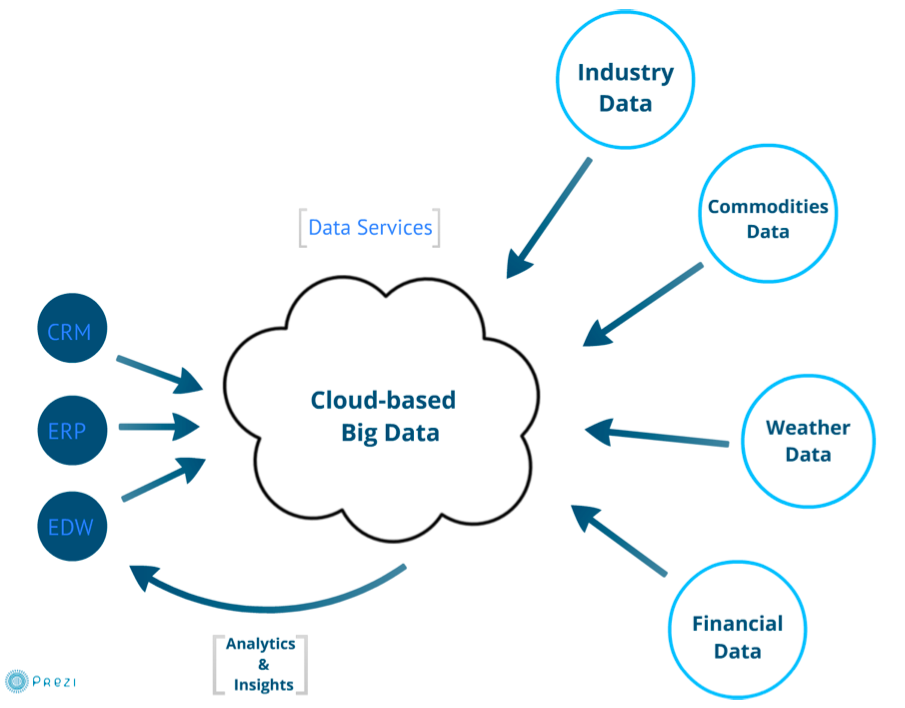
2.15.3 - e-Commerce and LifeStyle
e-Commerce and LifeStyle
Recommender systems operate under the hood of such widely recognized sites as Amazon, eBay, Monster and Netflix where everything is a recommendation. This involves a symbiotic relationship between vendor and buyer whereby the buyer provides the vendor with information about their preferences, while the vendor then offers recommendations tailored to match their needs. Kaggle competitions h improve the success of the Netflix and other recommender systems. Attention is paid to models that are used to compare how changes to the systems affect their overall performance. It is interesting that the humble ranking has become such a dominant driver of the world’s economy. More examples of recommender systems are given from Google News, Retail stores and in depth Yahoo! covering the multi-faceted criteria used in deciding recommendations on web sites.
The formulation of recommendations in terms of points in a space or bag is given where bags of item properties, user properties, rankings and users are useful. Detail is given on basic principles behind recommender systems: user-based collaborative filtering, which uses similarities in user rankings to predict their interests, and the Pearson correlation, used to statistically quantify correlations between users viewed as points in a space of items. Items are viewed as points in a space of users in item-based collaborative filtering. The Cosine Similarity is introduced, the difference between implicit and explicit ratings and the k Nearest Neighbors algorithm. General features like the curse of dimensionality in high dimensions are discussed. A simple Python k Nearest Neighbor code and its application to an artificial data set in 3 dimensions is given. Results are visualized in Matplotlib in 2D and with Plotviz in 3D. The concept of a training and a testing set are introduced with training set pre labeled. Recommender system are used to discuss clustering with k-means based clustering methods used and their results examined in Plotviz. The original labelling is compared to clustering results and extension to 28 clusters given. General issues in clustering are discussed including local optima, the use of annealing to avoid this and value of heuristic algorithms.
Recommender Systems
We introduce Recommender systems as an optimization technology used in a variety of applications and contexts online. They operate in the background of such widely recognized sites as Amazon, eBay, Monster and Netflix where everything is a recommendation. This involves a symbiotic relationship between vendor and buyer whereby the buyer provides the vendor with information about their preferences, while the vendor then offers recommendations tailored to match their needs, to the benefit of both.
There follows an exploration of the Kaggle competition site, other recommender systems and Netflix, as well as competitions held to improve the success of the Netflix recommender system. Finally attention is paid to models that are used to compare how changes to the systems affect their overall performance. It is interesting how the humble ranking has become such a dominant driver of the world’s economy.
Recommender Systems as an Optimization Problem
We define a set of general recommender systems as matching of items to people or perhaps collections of items to collections of people where items can be other people, products in a store, movies, jobs, events, web pages etc. We present this as “yet another optimization problem”.
Recommender Systems Introduction
We give a general discussion of recommender systems and point out that they are particularly valuable in long tail of tems (to be recommended) that are not commonly known. We pose them as a rating system and relate them to information retrieval rating systems. We can contrast recommender systems based on user profile and context; the most familiar collaborative filtering of others ranking; item properties; knowledge and hybrid cases mixing some or all of these.
Recommender Systems Introduction
(12:56)
Kaggle Competitions
We look at Kaggle competitions with examples from web site. In particular we discuss an Irvine class project involving ranking jokes.
Please not that we typically do not accept any projects using kaggle data for this classes. This class is not about winning a kaggle competition and if done wrong it does not fullfill the minimum requiremnt for this class. Please consult with the instructor.
Examples of Recommender Systems
We go through a list of 9 recommender systems from the same Irvine class.
Examples of Recommender Systems
(1:00)
Netflix on Recommender Systems
We summarize some interesting points from a tutorial from Netflix for whom everything is a recommendation. Rankings are given in multiple categories and categories that reflect user interests are especially important. Criteria used include explicit user preferences, implicit based on ratings and hybrid methods as well as freshness and diversity. Netflix tries to explain the rationale of its recommendations. We give some data on Netflix operations and some methods used in its recommender systems. We describe the famous Netflix Kaggle competition to improve its rating system. The analogy to maximizing click through rate is given and the objectives of optimization are given.
Netflix on Recommender Systems
(14:20)
Next we go through Netflix’s methodology in letting data speak for itself in optimizing the recommender engine. An example iis given on choosing self produced movies. A/B testing is discussed with examples showing how testing does allow optimizing of sophisticated criteria. This lesson is concluded by comments on Netflix technology and the full spectrum of issues that are involved including user interface, data, AB testing, systems and architectures. We comment on optimizing for a household rather than optimizing for individuals in household.
Other Examples of Recommender Systems
We continue the discussion of recommender systems and their use in e-commerce. More examples are given from Google News, Retail stores and in depth Yahoo! covering the multi-faceted criteria used in deciding recommendations on web sites. Then the formulation of recommendations in terms of points in a space or bag is given.
Here bags of item properties, user properties, rankings and users are useful. Then we go into detail on basic principles behind recommender systems: user-based collaborative filtering, which uses similarities in user rankings to predict their interests, and the Pearson correlation, used to statistically quantify correlations between users viewed as points in a space of items.
We start with a quick recap of recommender systems from previous unit; what they are with brief examples.
Recap and Examples of Recommender Systems
(5:48)
Examples of Recommender Systems
We give 2 examples in more detail: namely Google News and Markdown in Retail.
Examples of Recommender Systems
(8:34)
Recommender Systems in Yahoo Use Case Example
We describe in greatest detail the methods used to optimize Yahoo web sites. There are two lessons discussing general approach and a third lesson examines a particular personalized Yahoo page with its different components. We point out the different criteria that must be blended in making decisions; these criteria include analysis of what user does after a particular page is clicked; is the user satisfied and cannot that we quantified by purchase decisions etc. We need to choose Articles, ads, modules, movies, users, updates, etc to optimize metrics such as relevance score, CTR, revenue, engagement.These lesson stress that if though we have big data, the recommender data is sparse. We discuss the approach that involves both batch (offline) and on-line (real time) components.
Recap of Recommender Systems II
(8:46)
Recap of Recommender Systems III
(10:48)
Case Study of Recommender systems
(3:21)
User-based nearest-neighbor collaborative filtering
Collaborative filtering is a core approach to recommender systems. There is user-based and item-based collaborative filtering and here we discuss the user-based case. Here similarities in user rankings allow one to predict their interests, and typically this quantified by the Pearson correlation, used to statistically quantify correlations between users.
User-based nearest-neighbor collaborative filtering I
(7:20)
User-based nearest-neighbor collaborative filtering II
(7:29)
Vector Space Formulation of Recommender Systems
We go through recommender systems thinking of them as formulated in a funny vector space. This suggests using clustering to make recommendations.
Vector Space Formulation of Recommender Systems new
(9:06)
Resources
Item-based Collaborative Filtering and its Technologies
We move on to item-based collaborative filtering where items are viewed as points in a space of users. The Cosine Similarity is introduced, the difference between implicit and explicit ratings and the k Nearest Neighbors algorithm. General features like the curse of dimensionality in high dimensions are discussed.
Item-based Collaborative Filtering
We covered user-based collaborative filtering in the previous unit. Here we start by discussing memory-based real time and model based offline (batch) approaches. Now we look at item-based collaborative filtering where items are viewed in the space of users and the cosine measure is used to quantify distances. WE discuss optimizations and how batch processing can help. We discuss different Likert ranking scales and issues with new items that do not have a significant number of rankings.
k Nearest Neighbors and High Dimensional Spaces
(7:16)
k-Nearest Neighbors and High Dimensional Spaces
We define the k Nearest Neighbor algorithms and present the Python software but do not use it. We give examples from Wikipedia and describe performance issues. This algorithm illustrates the curse of dimensionality. If items were a real vectors in a low dimension space, there would be faster solution methods.
k Nearest Neighbors and High Dimensional Spaces
(10:03)
Recommender Systems - K-Neighbors
Next we provide some sample Python code for the k Nearest Neighbor and its application to an artificial data set in 3 dimensions. Results are visualized in Matplotlib in 2D and with Plotviz in 3D. The concept of training and testing sets are introduced with training set pre-labelled. This lesson is adapted from the Python k Nearest Neighbor code found on the web associated with a book by Harrington on Machine Learning [??]. There are two data sets. First we consider a set of 4 2D vectors divided into two categories (clusters) and use k=3 Nearest Neighbor algorithm to classify 3 test points. Second we consider a 3D dataset that has already been classified and show how to normalize. In this lesson we just use Matplotlib to give 2D plots.
The lesson goes through an example of using k NN classification algorithm by dividing dataset into 2 subsets. One is training set with initial classification; the other is test point to be classified by k=3 NN using training set. The code records fraction of points with a different classification from that input. One can experiment with different sizes of the two subsets. The Python implementation of algorithm is analyzed in detail.
Plotviz
The clustering methods are used and their results examined in Plotviz. The original labelling is compared to clustering results and extension to 28 clusters given. General issues in clustering are discussed including local optima, the use of annealing to avoid this and value of heuristic algorithms.
Files
- https://github.com/cloudmesh-community/book/blob/master/examples/python/knn/kNN.py
- https://github.com/cloudmesh-community/book/blob/master/examples/python/knn/kNN_Driver.py
- https://github.com/cloudmesh-community/book/blob/master/examples/python/knn/dating_test_set2.txt
- https://github.com/cloudmesh-community/book/blob/master/examples/python/knn/clusterFinal-M3-C3Dating-ReClustered.pviz
- https://github.com/cloudmesh-community/book/blob/master/examples/python/knn/dating_rating_original_labels.pviz
- https://github.com/cloudmesh-community/book/blob/master/examples/python/knn/clusterFinal-M30-C28.pviz
- https://github.com/cloudmesh-community/book/blob/master/examples/python/plotviz/clusterfinal_m3_c3dating_reclustered.pviz
- https://github.com/cloudmesh-community/book/blob/master/examples/python/plotviz/fungi_lsu_3_15_to_3_26_zeroidx.pviz
Resources k-means
- http://www.slideshare.net/xamat/building-largescale-realworld-recommender-systems-recsys2012-tutorial [@www-slideshare-building]
- http://www.ifi.uzh.ch/ce/teaching/spring2012/16-Recommender-Systems_Slides.pdf [@www-ifi-teaching]
- https://www.kaggle.com/ [@www-kaggle]
- http://www.ics.uci.edu/~welling/teaching/CS77Bwinter12/CS77B_w12.html [@www-ics-uci-welling]
- Jeff Hammerbacher[@20120117berkeley1]
- http://www.techworld.com/news/apps/netflix-foretells-house-of-cards-success-with-cassandra-big-data-engine-3437514/ [@www-techworld-netflix]
- https://en.wikipedia.org/wiki/A/B_testing [@wikipedia-ABtesting]
- http://www.infoq.com/presentations/Netflix-Architecture [@www-infoq-architec]
2.15.4 - Health Informatics
Health Informatics
This section starts by discussing general aspects of Big Data and Health including data sizes, different areas including genomics, EBI, radiology and the Quantified Self movement. We review current state of health care and trends associated with it including increased use of Telemedicine. We summarize an industry survey by GE and Accenture and an impressive exemplar Cloud-based medicine system from Potsdam. We give some details of big data in medicine. Some remarks on Cloud computing and Health focus on security and privacy issues.
We survey an April 2013 McKinsey report on the Big Data revolution in US health care; a Microsoft report in this area and a European Union report on how Big Data will allow patient centered care in the future. Examples are given of the Internet of Things, which will have great impact on health including wearables. A study looks at 4 scenarios for healthcare in 2032. Two are positive, one middle of the road and one negative. The final topic is Genomics, Proteomics and Information Visualization.
Big Data and Health
This lesson starts with general aspects of Big Data and Health including listing subareas where Big data important. Data sizes are given in radiology, genomics, personalized medicine, and the Quantified Self movement, with sizes and access to European Bioinformatics Institute.
Status of Healthcare Today
This covers trends of costs and type of healthcare with low cost genomes and an aging population. Social media and government Brain initiative.
Status of Healthcare Today
(16:09)
Telemedicine (Virtual Health)
This describes increasing use of telemedicine and how we tried and failed to do this in 1994.
Medical Big Data in the Clouds
An impressive exemplar Cloud-based medicine system from Potsdam.
Medical Big Data in the Clouds
(15:02)
Medical image Big Data
Clouds and Health
McKinsey Report on the big-data revolution in US health care
This lesson covers 9 aspects of the McKinsey report. These are the convergence of multiple positive changes has created a tipping point for
innovation; Primary data pools are at the heart of the big data revolution in healthcare; Big data is changing the paradigm: these are the value pathways; Applying early successes at scale could reduce US healthcare costs by $300 billion to $450 billion; Most new big-data applications target consumers and providers across pathways; Innovations are weighted towards influencing individual decision-making levers; Big data innovations use a range of public, acquired, and proprietary data
types; Organizations implementing a big data transformation should provide the leadership required for the associated cultural transformation; Companies must develop a range of big data capabilities.
Microsoft Report on Big Data in Health
This lesson identifies data sources as Clinical Data, Pharma & Life Science Data, Patient & Consumer Data, Claims & Cost Data and Correlational Data. Three approaches are Live data feed, Advanced analytics and Social analytics.
Microsoft Report on Big Data in Health
(2:26)
EU Report on Redesigning health in Europe for 2020
This lesson summarizes an EU Report on Redesigning health in Europe for 2020. The power of data is seen as a lever for change in My Data, My decisions; Liberate the data; Connect up everything; Revolutionize health; and Include Everyone removing the current correlation between health and wealth.
EU Report on Redesigning health in Europe for 2020
(5:00)
Medicine and the Internet of Things
The Internet of Things will have great impact on health including telemedicine and wearables. Examples are given.
Medicine and the Internet of Things
(8:17)
Extrapolating to 2032
A study looks at 4 scenarios for healthcare in 2032. Two are positive, one middle of the road and one negative.
Genomics, Proteomics and Information Visualization
A study of an Azure application with an Excel frontend and a cloud BLAST backend starts this lesson. This is followed by a big data analysis of personal genomics and an analysis of a typical DNA sequencing analytics pipeline. The Protein Sequence Universe is defined and used to motivate Multi dimensional Scaling MDS. Sammon’s method is defined and its use illustrated by a metagenomics example. Subtleties in use of MDS include a monotonic mapping of the dissimilarity function. The application to the COG Proteomics dataset is discussed. We note that the MDS approach is related to the well known chisq method and some aspects of nonlinear minimization of chisq (Least Squares) are discussed.
Genomics, Proteomics and Information Visualization
(6:56)
Next we continue the discussion of the COG Protein Universe introduced in the last lesson. It is shown how Proteomics clusters are clearly seen in the Universe browser. This motivates a side remark on different clustering methods applied to metagenomics. Then we discuss the Generative Topographic Map GTM method that can be used in dimension reduction when original data is in a metric space and is in this case faster than MDS as GTM computational complexity scales like N not N squared as seen in MDS.
Examples are given of GTM including an application to topic models in Information Retrieval. Indiana University has developed a deterministic annealing improvement of GTM. 3 separate clusterings are projected for visualization and show very different structure emphasizing the importance of visualizing results of data analytics. The final slide shows an application of MDS to generate and visualize phylogenetic trees.
\TODO{These two videos need to be uploaded to youtube}
Genomics, Proteomics and Information Visualization I
(10:33)
Genomics, Proteomics and Information Visualization: II
(7:41)
 Proteomics and Information Visualization
(131)
Proteomics and Information Visualization
(131)
Resources
- https://wiki.nci.nih.gov/display/CIP/CIP+Survey+of+Biomedical+Imaging+Archives [@wiki-nih-cip-survey]
- http://grids.ucs.indiana.edu/ptliupages/publications/Where\%20does\%20all\%20the\%20data\%20come\%20from\%20v7.pdf [@fox2011does]
http://www.ieee-icsc.org/ICSC2010/Tony\%20Hey\%20-\%2020100923.pdf(this link does not exist any longer)- http://quantifiedself.com/larry-smarr/ [@smarr13self]
- http://www.ebi.ac.uk/Information/Brochures/ [@www-ebi-aboutus]
- http://www.kpcb.com/internet-trends [@www-kleinerperkins-internet-trends]
- http://www.slideshare.net/drsteventucker/wearable-health-fitness-trackers-and-the-quantified-self [@www-slideshare-wearable-quantified-self]
- http://www.siam.org/meetings/sdm13/sun.pdf [@archive–big-data-analytics-healthcare]
- http://en.wikipedia.org/wiki/Calico_\%28company\%29 [@www-wiki-calico]
- http://www.slideshare.net/GSW_Worldwide/2015-health-trends [@www-slideshare-2015-health trends]
- http://www.accenture.com/SiteCollectionDocuments/PDF/Accenture-Industrial-Internet-Changing-Competitive-Landscape-Industries.pdf [@www-accenture-insight-industrial-internet]
- http://www.slideshare.net/schappy/how-realtime-analysis-turns-big-medical-data-into-precision-medicine [@www-slideshare-big-medical-data-medicine]
- http://medcitynews.com/2013/03/the-body-in-bytes-medical-images-as-a-source-of-healthcare-big-data-infographic/ [@medcitynews-bytes-medical-images]
http://healthinformatics.wikispaces.com/file/view/cloud_computing.ppt(this link does not exist any longer)- https://www.mckinsey.com/~/media/mckinsey/industries/healthcare%20systems%20and%20services/our%20insights/the%20big%20data%20revolution%20in%20us%20health%20care/the_big_data_revolution_in_healthcare.ashx [@www-mckinsey-industries-healthcare]
https://partner.microsoft.com/download/global/40193764(this link does not exist any longer)- https://ec.europa.eu/eip/ageing/file/353/download_en?token=8gECi1RO
http://www.liveathos.com/apparel/app- http://debategraph.org/Poster.aspx?aID=77 [@debategraph-poster]
http://www.oerc.ox.ac.uk/downloads/presentations-from-events/microsoftworkshop/gannon(this link does not exist any longer)http://www.delsall.org(this link does not exist any longer)- http://salsahpc.indiana.edu/millionseq/mina/16SrRNA_index.html [@www-salsahpc-millionseq]
- http://www.geatbx.com/docu/fcnindex-01.html [@www-geatbx-parametric-optimization]
2.15.5 - Overview of Data Science
Overview of Data Science
What is Big Data, Data Analytics and X-Informatics?
We start with X-Informatics and its rallying cry. The growing number of jobs in data science is highlighted. The first unit offers a look at the phenomenon described as the Data Deluge starting with its broad features. Data science and the famous DIKW (Data to Information to Knowledge to Wisdom) pipeline are covered. Then more detail is given on the flood of data from Internet and Industry applications with eBay and General Electric discussed in most detail.
In the next unit, we continue the discussion of the data deluge with a focus on scientific research. He takes a first peek at data from the Large Hadron Collider considered later as physics Informatics and gives some biology examples. He discusses the implication of data for the scientific method which is changing with the data-intensive methodology joining observation, theory and simulation as basic methods. Two broad classes of data are the long tail of sciences: many users with individually modest data adding up to a lot; and a myriad of Internet connected devices – the Internet of Things.
We give an initial technical overview of cloud computing as pioneered by companies like Amazon, Google and Microsoft with new centers holding up to a million servers. The benefits of Clouds in terms of power consumption and the environment are also touched upon, followed by a list of the most critical features of Cloud computing with a comparison to supercomputing. Features of the data deluge are discussed with a salutary example where more data did better than more thought. Then comes Data science and one part of it ~~ data analytics ~~ the large algorithms that crunch the big data to give big wisdom. There are many ways to describe data science and several are discussed to give a good composite picture of this emerging field.
Data Science generics and Commercial Data Deluge
We start with X-Informatics and its rallying cry. The growing number of jobs in data science is highlighted. This unit offers a look at the phenomenon described as the Data Deluge starting with its broad features. Then he discusses data science and the famous DIKW (Data to Information to Knowledge to Wisdom) pipeline. Then more detail is given on the flood of data from Internet and Industry applications with eBay and General Electric discussed in most detail.
What is X-Informatics and its Motto
This discusses trends that are driven by and accompany Big data. We give some key terms including data, information, knowledge, wisdom, data analytics and data science. We discuss how clouds running Data Analytics Collaboratively processing Big Data can solve problems in X-Informatics. We list many values of X you can defined in various activities across the world.
Jobs
Big data is especially important as there are some many related jobs. We illustrate this for both cloud computing and data science from reports by Microsoft and the McKinsey institute respectively. We show a plot from LinkedIn showing rapid increase in the number of data science and analytics jobs as a function of time.
Data Deluge: General Structure
We look at some broad features of the data deluge starting with the size of data in various areas especially in science research. We give examples from real world of the importance of big data and illustrate how it is integrated into an enterprise IT architecture. We give some views as to what characterizes Big data and why data science is a science that is needed to interpret all the data.
Data Science: Process
We stress the DIKW pipeline: Data becomes information that becomes knowledge and then wisdom, policy and decisions. This pipeline is illustrated with Google maps and we show how complex the ecosystem of data, transformations (filters) and its derived forms is.
Data Deluge: Internet
We give examples of Big data from the Internet with Tweets, uploaded photos and an illustration of the vitality and size of many commodity applications.
Data Deluge: Business
We give examples including the Big data that enables wind farms, city transportation, telephone operations, machines with health monitors, the banking, manufacturing and retail industries both online and offline in shopping malls. We give examples from ebay showing how analytics allowing them to refine and improve the customer experiences.
Resources
- http://www.microsoft.com/en-us/news/features/2012/mar12/03-05CloudComputingJobs.aspx
- http://www.mckinsey.com/mgi/publications/big_data/index.asp
- Tom Davenport
- Anjul Bhambhri
- Jeff Hammerbacher
- http://www.economist.com/node/15579717
- http://cs.metrostate.edu/~sbd/slides/Sun.pdf
- http://jess3.com/geosocial-universe-2/
- Bill Ruh
- http://www.hsph.harvard.edu/ncb2011/files/ncb2011-z03-rodriguez.pptx
- Hugh Williams
Data Deluge and Scientific Applications and Methodology
Overview of Data Science
We continue the discussion of the data deluge with a focus on scientific research. He takes a first peek at data from the Large Hadron Collider considered later as physics Informatics and gives some biology examples. He discusses the implication of data for the scientific method which is changing with the data-intensive methodology joining observation, theory and simulation as basic methods. We discuss the long tail of sciences; many users with individually modest data adding up to a lot. The last lesson emphasizes how everyday devices ~~ the Internet of Things ~~ are being used to create a wealth of data.
Science and Research
We look into more big data examples with a focus on science and research. We give astronomy, genomics, radiology, particle physics and discovery of Higgs particle (Covered in more detail in later lessons), European Bioinformatics Institute and contrast to Facebook and Walmart.
Implications for Scientific Method
We discuss the emergencies of a new fourth methodology for scientific research based on data driven inquiry. We contrast this with third ~~ computation or simulation based discovery - methodology which emerged itself some 25 years ago.
Long Tail of Science
There is big science such as particle physics where a single experiment has 3000 people collaborate!.Then there are individual investigators who do not generate a lot of data each but together they add up to Big data.
Internet of Things
A final category of Big data comes from the Internet of Things where lots of small devices ~~ smart phones, web cams, video games collect and disseminate data and are controlled and coordinated in the cloud.
Resources
- http://www.economist.com/node/15579717
- Geoffrey Fox and Dennis Gannon Using Clouds for Technical Computing To be published in Proceedings of HPC 2012 Conference at Cetraro, Italy June 28 2012
- http://grids.ucs.indiana.edu/ptliupages/publications/Clouds_Technical_Computing_FoxGannonv2.pdf
- http://grids.ucs.indiana.edu/ptliupages/publications/Where%20does%20all%20the%20data%20come%20from%20v7.pdf
- http://www.genome.gov/sequencingcosts/
- http://www.quantumdiaries.org/2012/09/07/why-particle-detectors-need-a-trigger/atlasmgg
- http://salsahpc.indiana.edu/dlib/articles/00001935/
- http://en.wikipedia.org/wiki/Simple_linear_regression
- http://www.ebi.ac.uk/Information/Brochures/
- http://www.wired.com/wired/issue/16-07
- http://research.microsoft.com/en-us/collaboration/fourthparadigm/
- CSTI General Assembly 2012, Washington, D.C., USA Technical Activities Coordinating Committee (TACC) Meeting, Data Management, Cloud Computing and the Long Tail of Science October 2012 Dennis Gannon
Clouds and Big Data Processing; Data Science Process and Analytics
Overview of Data Science
We give an initial technical overview of cloud computing as pioneered by companies like Amazon, Google and Microsoft with new centers holding up to a million servers. The benefits of Clouds in terms of power consumption and the environment are also touched upon, followed by a list of the most critical features of Cloud computing with a comparison to supercomputing.
He discusses features of the data deluge with a salutary example where more data did better than more thought. He introduces data science and one part of it ~~ data analytics ~~ the large algorithms that crunch the big data to give big wisdom. There are many ways to describe data science and several are discussed to give a good composite picture of this emerging field.
Clouds
We describe cloud data centers with their staggering size with up to a million servers in a single data center and centers built modularly from shipping containers full of racks. The benefits of Clouds in terms of power consumption and the environment are also touched upon, followed by a list of the most critical features of Cloud computing and a comparison to supercomputing.
- Clouds
(16:04){MP4}
Aspect of Data Deluge
Data, Information, intelligence algorithms, infrastructure, data structure, semantics and knowledge are related. The semantic web and Big data are compared. We give an example where “More data usually beats better algorithms”. We discuss examples of intelligent big data and list 8 different types of data deluge
Data Science Process
We describe and critique one view of the work of a data scientists. Then we discuss and contrast 7 views of the process needed to speed data through the DIKW pipeline.
Data Analytics
Data Analytics
(30)
We stress the importance of data analytics givi ng examples from several
fields. We note that better analytics is as important as better
computing and storage capability. In the second video we look at High
Performance Computing in Science and Engineering: the Tree and the
Fruit.
Resources
- CSTI General Assembly 2012, Washington, D.C., USA Technical Activities Coordinating Committee (TACC) Meeting, Data Management, Cloud Computing and the Long Tail of Science October 2012 Dennis Gannon
- Dan Reed Roger Barga Dennis Gannon Rich Wolski http://research.microsoft.com/en-us/people/barga/sc09\_cloudcomp_tutorial.pdf
- http://www.datacenterknowledge.com/archives/2011/05/10/uptime-institute-the-average-pue-is-1-8/
- http://loosebolts.wordpress.com/2008/12/02/our-vision-for-generation-4-modular-data-centers-one-way-of-getting-it-just-right/
- http://www.mediafire.com/file/zzqna34282frr2f/koomeydatacenterelectuse2011finalversion.pdf
- Bina Ramamurthy
- Jeff Hammerbacher
- Jeff Hammerbacher
- Anjul Bhambhri
- http://cs.metrostate.edu/~sbd/slides/Sun.pdf
- Hugh Williams
- Tom Davenport
- http://www.mckinsey.com/mgi/publications/big_data/index.asp
- http://cra.org/ccc/docs/nitrdsymposium/pdfs/keyes.pdf
2.15.6 - Physics
Physics
This section starts by describing the LHC accelerator at CERN and evidence found by the experiments suggesting existence of a Higgs Boson. The huge number of authors on a paper, remarks on histograms and Feynman diagrams is followed by an accelerator picture gallery. The next unit is devoted to Python experiments looking at histograms of Higgs Boson production with various forms of shape of signal and various background and with various event totals. Then random variables and some simple principles of statistics are introduced with explanation as to why they are relevant to Physics counting experiments. The unit introduces Gaussian (normal) distributions and explains why they seen so often in natural phenomena. Several Python illustrations are given. Random Numbers with their Generators and Seeds lead to a discussion of Binomial and Poisson Distribution. Monte-Carlo and accept-reject methods. The Central Limit Theorem concludes discussion.
Looking for Higgs Particles
Bumps in Histograms, Experiments and Accelerators
This unit is devoted to Python and Java experiments looking at histograms of Higgs Boson production with various forms of shape of signal and various background and with various event totals. The lectures use Python but use of Java is described.
-
<{gitcode}/physics/mr-higgs/higgs-classI-sloping.py>
Particle Counting
We return to particle case with slides used in introduction and stress that particles often manifested as bumps in histograms and those bumps need to be large enough to stand out from background in a statistically significant fashion.
We give a few details on one LHC experiment ATLAS. Experimental physics papers have a staggering number of authors and quite big budgets. Feynman diagrams describe processes in a fundamental fashion.
Experimental Facilities
We give a few details on one LHC experiment ATLAS. Experimental physics papers have a staggering number of authors and quite big budgets. Feynman diagrams describe processes in a fundamental fashion.
Accelerator Picture Gallery of Big Science
This lesson gives a small picture gallery of accelerators. Accelerators, detection chambers and magnets in tunnels and a large underground laboratory used fpr experiments where you need to be shielded from background like cosmic rays.
Resources
- http://grids.ucs.indiana.edu/ptliupages/publications/Where%20does%20all%20the%20data%20come%20from%20v7.pdf [@fox2011does]
- http://www.sciencedirect.com/science/article/pii/S037026931200857X [@aad2012observation]
- http://www.nature.com/news/specials/lhc/interactive.html
Looking for Higgs Particles: Python Event Counting for Signal and Background (Part 2)
This unit is devoted to Python experiments looking at histograms of Higgs Boson production with various forms of shape of signal and various background and with various event totals.
Files:
- <{gitcode}/physics/mr-higgs/higgs-classI-sloping.py>
- <{gitcode}/physics/number-theory/higgs-classIII.py>
- <{gitcode}/physics/mr-higgs/higgs-classII-uniform.py>
Event Counting
We define event counting data collection environments. We discuss the python and Java code to generate events according to a particular scenario (the important idea of Monte Carlo data). Here a sloping background plus either a Higgs particle generated similarly to LHC observation or one observed with better resolution (smaller measurement error).
Monte Carlo
This uses Monte Carlo data both to generate data like the experimental observations and explore effect of changing amount of data and changing measurement resolution for Higgs.
-
With Python examples of Signal plus Background
(7:33) This lesson continues the
examination of Monte Carlo data looking at effect of change in
number of Higgs particles produced and in change in shape of
background.
Resources
- Python for Data Analysis: Agile Tools for Real World Data By Wes McKinney, Publisher: O’Reilly Media, Released: October 2012, Pages: 472. [@mckinney-python]
- http://jwork.org/scavis/api/ [@jwork-api]
- https://en.wikipedia.org/wiki/DataMelt [@wikipedia-datamelt]
Random Variables, Physics and Normal Distributions
We introduce random variables and some simple principles of statistics and explains why they are relevant to Physics counting experiments. The unit introduces Gaussian (normal) distributions and explains why they seen so often in natural phenomena. Several Python illustrations are given. Java is currently not available in this unit.
-
Higgs (39)
- <{gitcode}/physics/number-theory/higgs-classIII.py>
Statistics Overview and Fundamental Idea: Random Variables
We go through the many different areas of statistics covered in the Physics unit. We define the statistics concept of a random variable.
Physics and Random Variables
We describe the DIKW pipeline for the analysis of this type of physics experiment and go through details of analysis pipeline for the LHC ATLAS experiment. We give examples of event displays showing the final state particles seen in a few events. We illustrate how physicists decide whats going on with a plot of expected Higgs production experimental cross sections (probabilities) for signal and background.
Statistics of Events with Normal Distributions
We introduce Poisson and Binomial distributions and define independent identically distributed (IID) random variables. We give the law of large numbers defining the errors in counting and leading to Gaussian distributions for many things. We demonstrate this in Python experiments.
Gaussian Distributions
We introduce the Gaussian distribution and give Python examples of the fluctuations in counting Gaussian distributions.
Using Statistics
We discuss the significance of a standard deviation and role of biases and insufficient statistics with a Python example in getting incorrect answers.
Resources
- http://indico.cern.ch/event/20453/session/6/contribution/15?materialId=slides
http://www.atlas.ch/photos/events.html(this link is outdated)- https://cms.cern/ [@cms]
Random Numbers, Distributions and Central Limit Theorem
We discuss Random Numbers with their Generators and Seeds. It introduces Binomial and Poisson Distribution. Monte-Carlo and accept-reject methods are discussed. The Central Limit Theorem and Bayes law concludes discussion. Python and Java (for student - not reviewed in class) examples and Physics applications are given.
Files:
- <{gitcode}/physics/calculated-dice-roll/higgs-classIV-seeds.py>
Generators and Seeds
We define random numbers and describe how to generate them on the computer giving Python examples. We define the seed used to define to specify how to start generation.
Binomial Distribution
We define binomial distribution and give LHC data as an example of where this distribution valid.
Accept-Reject
We introduce an advanced method accept/reject for generating random variables with arbitrary distributions.
Monte Carlo Method
We define Monte Carlo method which usually uses accept/reject method in typical case for distribution.
Poisson Distribution
We extend the Binomial to the Poisson distribution and give a set of amusing examples from Wikipedia.
Central Limit Theorem
We introduce Central Limit Theorem and give examples from Wikipedia.
Interpretation of Probability: Bayes v. Frequency
This lesson describes difference between Bayes and frequency views of probability. Bayes’s law of conditional probability is derived and applied to Higgs example to enable information about Higgs from multiple channels and multiple experiments to be accumulated.
Resources
\TODO{integrate physics-references.bib}
SKA – Square Kilometer Array
Professor Diamond, accompanied by Dr. Rosie Bolton from the SKA Regional Centre Project gave a presentation at SC17 “into the deepest reaches of the observable universe as they describe the SKA’s international partnership that will map and study the entire sky in greater detail than ever before.”
A summary article about this effort is available at:
- https://www.hpcwire.com/2017/11/17/sc17-keynote-hpc-powers-ska-efforts-peer-deep-cosmos/ The video is hosted at
- http://sc17.supercomputing.org/presentation/?id=inspkr101&sess=sess263 Start at about 1:03:00 (e.g. the one hour mark)
2.15.7 - Plotviz
Plotviz
NOTE: This an legacy application this has now been replaced by WebPlotViz which is a web browser based visualization tool which provides added functionality’s.
We introduce Plotviz, a data visualization tool developed at Indiana University to display 2 and 3 dimensional data. The motivation is that the human eye is very good at pattern recognition and can see structure in data. Although most Big data is higher dimensional than 3, all can be transformed by dimension reduction techniques to 3D. He gives several examples to show how the software can be used and what kind of data can be visualized. This includes individual plots and the manipulation of multiple synchronized plots.Finally, he describes the download and software dependency of Plotviz.
Using Plotviz Software for Displaying Point Distributions in 3D
We introduce Plotviz, a data visualization tool developed at Indiana University to display 2 and 3 dimensional data. The motivation is that the human eye is very good at pattern recognition and can see structure in data. Although most Big data is higher dimensional than 3, all can be transformed by dimension reduction techniques to 3D. He gives several examples to show how the software can be used and what kind of data can be visualized. This includes individual plots and the manipulation of multiple synchronized plots. Finally, he describes the download and software dependency of Plotviz.
Files:
- https://github.com/cloudmesh-community/book/blob/master/examples/python/plotviz/fungi-lsu-3-15-to-3-26-zeroidx.pviz
- https://github.com/cloudmesh-community/book/blob/master/examples/python/plotviz/datingrating-originallabels.pviz
- https://github.com/cloudmesh-community/book/blob/master/examples/python/plotviz/clusterFinal-M30-C28.pviz
- https://github.com/cloudmesh-community/book/blob/master/examples/python/plotviz/clusterfinal-m3-c3dating-reclustered.pviz
Motivation and Introduction to use
The motivation of Plotviz is that the human eye is very good at pattern recognition and can see structure in data. Although most Big data is higher dimensional than 3, all data can be transformed by dimension reduction techniques to 3D and one can check analysis like clustering and/or see structure missed in a computer analysis. The motivations shows some Cheminformatics examples. The use of Plotviz is started in slide 4 with a discussion of input file which is either a simple text or more features (like colors) can be specified in a rich XML syntax. Plotviz deals with points and their classification (clustering). Next the protein sequence browser in 3D shows the basic structure of Plotviz interface. The next two slides explain the core 3D and 2D manipulations respectively. Note all files used in examples are available to students.
Example of Use I: Cube and Structured Dataset
Initially we start with a simple plot of 8 points – the corners of a cube in 3 dimensions – showing basic operations such as size/color/labels and Legend of points. The second example shows a dataset (coming from GTM dimension reduction) with significant structure. This has .pviz and a .txt versions that are compared.
Example of Use II: Proteomics and Synchronized Rotation
This starts with an examination of a sample of Protein Universe Browser showing how one uses Plotviz to look at different features of this set of Protein sequences projected to 3D. Then we show how to compare two datasets with synchronized rotation of a dataset clustered in 2 different ways; this dataset comes from k Nearest Neighbor discussion.
Proteomics and Synchronized Rotation (9:14)
Example of Use III: More Features and larger Proteomics Sample
This starts by describing use of Labels and Glyphs and the Default mode in Plotviz. Then we illustrate sophisticated use of these ideas to view a large Proteomics dataset.
Larger Proteomics Sample (8:37)
Example of Use IV: Tools and Examples
This lesson starts by describing the Plotviz tools and then sets up two examples – Oil Flow and Trading – described in PowerPoint. It finishes with the Plotviz viewing of Oil Flow data.
Example of Use V: Final Examples
This starts with Plotviz looking at Trading example introduced in previous lesson and then examines solvent data. It finishes with two large biology examples with 446K and 100K points and each with over 100 clusters. We finish remarks on Plotviz software structure and how to download. We also remind you that a picture is worth a 1000 words.
Resources
2.15.8 - Practical K-Means, Map Reduce, and Page Rank for Big Data Applications and Analytics
Practical K-Means, Map Reduce, and Page Rank for Big Data Applications and Analytics
We use the K-means Python code in SciPy package to show real code for clustering. After a simple example we generate 4 clusters of distinct centers and various choice for sizes using Matplotlib tor visualization. We show results can sometimes be incorrect and sometimes make different choices among comparable solutions. We discuss the hill between different solutions and rationale for running K-means many times and choosing best answer. Then we introduce MapReduce with the basic architecture and a homely example. The discussion of advanced topics includes an extension to Iterative MapReduce from Indiana University called Twister and a generalized Map Collective model. Some measurements of parallel performance are given. The SciPy K-means code is modified to support a MapReduce execution style. This illustrates the key ideas of mappers and reducers. With appropriate runtime this code would run in parallel but here the parallel maps run sequentially. This simple 2 map version can be generalized to scalable parallelism. Python is used to Calculate PageRank from Web Linkage Matrix showing several different formulations of the basic matrix equations to finding leading eigenvector. The unit is concluded by a calculation of PageRank for general web pages by extracting the secret from Google.
K-means in Practice
We introduce the k means algorithm in a gentle fashion and describes its key features including dangers of local minima. A simple example from Wikipedia is examined.
We use the K-means Python code in SciPy package to show real code for clustering. After a simple example we generate 4 clusters of distinct centers and various choice for sizes using Matplotlib tor visualization. We show results can sometimes be incorrect and sometimes make different choices among comparable solutions. We discuss the hill between different solutions and rationale for running K-means many times and choosing best answer.
Files:
- https://github.com/cloudmesh-community/book/blob/master/examples/python/kmeans/xmean.py
- https://github.com/cloudmesh-community/book/blob/master/examples/python/kmeans/sample.csv
- https://github.com/cloudmesh-community/book/blob/master/examples/python/kmeans/parallel-kmeans.py
- https://github.com/cloudmesh-community/book/blob/master/examples/python/kmeans/kmeans-extra.py
K-means in Python
We use the K-means Python code in SciPy package to show real code for clustering and applies it a set of 85 two dimensional vectors – officially sets of weights and heights to be clustered to find T-shirt sizes. We run through Python code with Matplotlib displays to divide into 2-5 clusters. Then we discuss Python to generate 4 clusters of varying sizes and centered at corners of a square in two dimensions. We formally give the K means algorithm better than before and make definition consistent with code in SciPy.
Analysis of 4 Artificial Clusters
We present clustering results on the artificial set of 1000 2D points described in previous lesson for 3 choices of cluster sizes small large and very large. We emphasize the SciPy always does 20 independent K means and takes the best result – an approach to avoiding local minima. We allow this number of independent runs to be changed and in particular set to 1 to generate more interesting erratic results. We define changes in our new K means code that also has two measures of quality allowed. The slides give many results of clustering into 2 4 6 and 8 clusters (there were only 4 real clusters). We show that the very small case has two very different solutions when clustered into two clusters and use this to discuss functions with multiple minima and a hill between them. The lesson has both discussion of already produced results in slides and interactive use of Python for new runs.
Parallel K-means
We modify the SciPy K-means code to support a MapReduce execution style and runs it in this short unit. This illustrates the key ideas of mappers and reducers. With appropriate runtime this code would run in parallel but here the parallel maps run sequentially. We stress that this simple 2 map version can be generalized to scalable parallelism.
Files:
PageRank in Practice
We use Python to Calculate PageRank from Web Linkage Matrix showing several different formulations of the basic matrix equations to finding leading eigenvector. The unit is concluded by a calculation of PageRank for general web pages by extracting the secret from Google.
Files:
- https://github.com/cloudmesh-community/book/blob/master/examples/python/page-rank/pagerank1.py
- https://github.com/cloudmesh-community/book/blob/master/examples/python/page-rank/pagerank2.py
Resources
2.15.9 - Radar
Radar
The changing global climate is suspected to have long-term effects on much of the world’s inhabitants. Among the various effects, the rising sea level will directly affect many people living in low-lying coastal regions. While the ocean-s thermal expansion has been the dominant contributor to rises in sea level, the potential contribution of discharges from the polar ice sheets in Greenland and Antarctica may provide a more significant threat due to the unpredictable response to the changing climate. The Radar-Informatics unit provides a glimpse in the processes fueling global climate change and explains what methods are used for ice data acquisitions and analysis.
Introduction
This lesson motivates radar-informatics by building on previous discussions on why X-applications are growing in data size and why analytics are necessary for acquiring knowledge from large data. The lesson details three mosaics of a changing Greenland ice sheet and provides a concise overview to subsequent lessons by detailing explaining how other remote sensing technologies, such as the radar, can be used to sound the polar ice sheets and what we are doing with radar images to extract knowledge to be incorporated into numerical models.
Remote Sensing
This lesson explains the basics of remote sensing, the characteristics of remote sensors and remote sensing applications. Emphasis is on image acquisition and data collection in the electromagnetic spectrum.
Ice Sheet Science
This lesson provides a brief understanding on why melt water at the base of the ice sheet can be detrimental and why it’s important for sensors to sound the bedrock.
Global Climate Change
This lesson provides an understanding and the processes for the greenhouse effect, how warming effects the Polar Regions, and the implications of a rise in sea level.
Radio Overview
This lesson provides an elementary introduction to radar and its importance to remote sensing, especially to acquiring information about Greenland and Antarctica.
Radio Informatics
This lesson focuses on the use of sophisticated computer vision algorithms, such as active contours and a hidden markov model to support data analysis for extracting layers, so ice sheet models can accurately forecast future changes in climate.
2.15.10 - Sensors
Sensors
We start with the Internet of Things IoT giving examples like monitors of machine operation, QR codes, surveillance cameras, scientific sensors, drones and self driving cars and more generally transportation systems. We give examples of robots and drones. We introduce the Industrial Internet of Things IIoT and summarize surveys and expectations Industry wide. We give examples from General Electric. Sensor clouds control the many small distributed devices of IoT and IIoT. More detail is given for radar data gathered by sensors; ubiquitous or smart cities and homes including U-Korea; and finally the smart electric grid.
Internet of Things
There are predicted to be 24-50 Billion devices on the Internet by 2020; these are typically some sort of sensor defined as any source or sink of time series data. Sensors include smartphones, webcams, monitors of machine operation, barcodes, surveillance cameras, scientific sensors (especially in earth and environmental science), drones and self driving cars and more generally transportation systems. The lesson gives many examples of distributed sensors, which form a Grid that is controlled by a cloud.
Robotics and IoT
Examples of Robots and Drones.
Robotics and IoT Expectations (8:05)
Industrial Internet of Things
We summarize surveys and expectations Industry wide.
Industrial Internet of Things (24:02)
Sensor Clouds
We describe the architecture of a Sensor Cloud control environment and gives example of interface to an older version of it. The performance of system is measured in terms of processing latency as a function of number of involved sensors with each delivering data at 1.8 Mbps rate.
Earth/Environment/Polar Science data gathered by Sensors
This lesson gives examples of some sensors in the Earth/Environment/Polar Science field. It starts with material from the CReSIS polar remote sensing project and then looks at the NSF Ocean Observing Initiative and NASA’s MODIS or Moderate Resolution Imaging Spectroradiometer instrument on a satellite.
Earth/Environment/Polar Science data gathered by Sensors
(4:58)
Ubiquitous/Smart Cities
For Ubiquitous/Smart cities we give two examples: Iniquitous Korea and smart electrical grids.
Ubiquitous/Smart Cities (1:44)
U-Korea (U=Ubiquitous)
Korea has an interesting positioning where it is first worldwide in broadband access per capita, e-government, scientific literacy and total working hours. However it is far down in measures like quality of life and GDP. U-Korea aims to improve the latter by Pervasive computing, everywhere, anytime i.e. by spreading sensors everywhere. The example of a ‘High-Tech Utopia’ New Songdo is given.
Smart Grid
The electrical Smart Grid aims to enhance USA’s aging electrical infrastructure by pervasive deployment of sensors and the integration of their measurement in a cloud or equivalent server infrastructure. A variety of new instruments include smart meters, power monitors, and measures of solar irradiance, wind speed, and temperature. One goal is autonomous local power units where good use is made of waste heat.
Resources
\TODO{These resources have not all been checked to see if they still exist this is currently in progress}
-
http://www.accenture.com/SiteCollectionDocuments/PDF/Accenture-Industrial-Internet-Changing-Competitive-Landscape-Industries.pdf [@www-accenture-insight-industrial]
-
http://www.gesoftware.com/ge-predictivity-infographic [@www-predix-ge-Industrial]
-
http://www.getransportation.com/railconnect360/rail-landscape [@www-getransportation-digital]
-
http://www.gesoftware.com/sites/default/files/GE-Software-Modernizing-Machine-to-Machine-Interactions.pdf [@www-ge-digital-software]
These resources do not exsit:
-
https://www.gesoftware.com/sites/default/files/the-industrial-internet/index.html
2.15.11 - Sports
Sports
Sports sees significant growth in analytics with pervasive statistics shifting to more sophisticated measures. We start with baseball as game is built around segments dominated by individuals where detailed (video/image) achievement measures including PITCHf/x and FIELDf/x are moving field into big data arena. There are interesting relationships between the economics of sports and big data analytics. We look at Wearables and consumer sports/recreation. The importance of spatial visualization is discussed. We look at other Sports: Soccer, Olympics, NFL Football, Basketball, Tennis and Horse Racing.
Basic Sabermetrics
This unit discusses baseball starting with the movie Moneyball and the 2002-2003 Oakland Athletics. Unlike sports like basketball and soccer, most baseball action is built around individuals often interacting in pairs. This is much easier to quantify than many player phenomena in other sports. We discuss Performance-Dollar relationship including new stadiums and media/advertising. We look at classic baseball averages and sophisticated measures like Wins Above Replacement.
Introduction and Sabermetrics (Baseball Informatics) Lesson
Introduction to all Sports Informatics, Moneyball The 2002-2003 Oakland Athletics, Diamond Dollars economic model of baseball, Performance - Dollar relationship, Value of a Win.
Introduction and Sabermetrics (Baseball Informatics) Lesson
(31:4)
Basic Sabermetrics
Different Types of Baseball Data, Sabermetrics, Overview of all data, Details of some statistics based on basic data, OPS, wOBA, ERA, ERC, FIP, UZR.
Wins Above Replacement
Wins above Replacement WAR, Discussion of Calculation, Examples, Comparisons of different methods, Coefficient of Determination, Another, Sabermetrics Example, Summary of Sabermetrics.
Wins Above Replacement
(30:43)
Advanced Sabermetrics
This unit discusses ‘advanced sabermetrics’ covering advances possible from using video from PITCHf/X, FIELDf/X, HITf/X, COMMANDf/X and MLBAM.
Pitching Clustering
A Big Data Pitcher Clustering method introduced by Vince Gennaro, Data from Blog and video at 2013 SABR conference.
Pitcher Quality
Results of optimizing match ups, Data from video at 2013 SABR conference.
PITCHf/X
Examples of use of PITCHf/X.
Other Video Data Gathering in Baseball
FIELDf/X, MLBAM, HITf/X, COMMANDf/X.
Other Video Data Gathering in Baseball
(18:5) Other Sports
We look at Wearables and consumer sports/recreation. The importance of spatial visualization is discussed. We look at other Sports: Soccer, Olympics, NFL Football, Basketball, Tennis and Horse Racing.
Wearables
Consumer Sports, Stake Holders, and Multiple Factors.
Soccer and the Olympics
Soccer, Tracking Players and Balls, Olympics.
Soccer and the Olympics
(8:28)
Spatial Visualization in NFL and NBA
NFL, NBA, and Spatial Visualization.
Spatial Visualization in NFL and NBA
(15:19)
Tennis and Horse Racing
Tennis, Horse Racing, and Continued Emphasis on Spatial Visualization.
Tennis and Horse Racing
(8:52)
Resources
\TODO{These resources have not all been checked to see if they still exist this is currently in progress}
-
http://www.slideshare.net/Tricon_Infotech/big-data-for-big-sports [@www-slideshare-tricon-infotech]
-
http://www.slideshare.net/BrandEmotivity/sports-analytics-innovation-summit-data-powered-storytelling [@www-slideshare-sports]
-
http://www.slideshare.net/elew/sport-analytics-innovation [@www-slideshare-elew-sport-analytics]
-
http://www.wired.com/2013/02/catapault-smartball/ [@www-wired-smartball]
-
http://www.sloansportsconference.com/wp-content/uploads/2014/06/Automated_Playbook_Generation.pdf [@www-sloansportsconference-automated-playbook]
-
http://autoscout.adsc.illinois.edu/publications/football-trajectory-dataset/ [@www-autoscout-illinois-football-trajectory]
-
http://www.sloansportsconference.com/wp-content/uploads/2012/02/Goldsberry_Sloan_Submission.pdf [@sloansportconference-goldsberry]
-
http://gamesetmap.com/ [@gamesetmap]
-
http://www.slideshare.net/BrandEmotivity/sports-analytics-innovation-summit-data-powered-storytelling [@www-slideshare-sports-datapowered]
-
http://www.sloansportsconference.com/ [@www-sloansportsconferences]
-
http://sabr.org/ [@www-sabr]
-
http://en.wikipedia.org/wiki/Sabermetrics [@wikipedia-Sabermetrics]
-
http://en.wikipedia.org/wiki/Baseball_statistics [@www-wikipedia-baseball-statistics]
-
http://m.mlb.com/news/article/68514514/mlbam-introduces-new-way-to-analyze-every-play [@www-mlb-mlbam-new-way-play]
-
http://www.fangraphs.com/library/offense/offensive-statistics-list/ [@www-fangraphs-offensive-statistics]
-
http://en.wikipedia.org/wiki/Component_ERA [@www-wiki-component-era]
-
http://www.fangraphs.com/library/pitching/fip/ [@www-fangraphs-pitching-fip]
-
http://en.wikipedia.org/wiki/Wins_Above_Replacement [@www-wiki-wins-above-replacement]
-
http://www.fangraphs.com/library/misc/war/ [@www-fangraphs-library-war]
-
http://www.baseball-reference.com/about/war_explained.shtml [@www-baseball-references-war-explained]
-
http://www.baseball-reference.com/about/war_explained_comparison.shtml [@www-baseball-references-war-explained-comparison]
-
http://www.baseball-reference.com/about/war_explained_position.shtml [@www-baseball-reference-war-explained-position]
-
http://www.baseball-reference.com/about/war_explained_pitch.shtml [@www-baseball-reference-war-explained-pitch]
-
http://www.fangraphs.com/leaders.aspx?pos=all&stats=bat&lg=all&qual=y&type=8&season=2014&month=0&season1=1871&ind=0 [@www-fangraphs-leaders-pose-qual]
-
http://battingleadoff.com/2014/01/08/comparing-the-three-war-measures-part-ii/ [@battingleadoff-baseball-player]
-
http://en.wikipedia.org/wiki/Coefficient_of_determination [@www-wiki-coefficient-of-determination]
-
http://www.sloansportsconference.com/wp-content/uploads/2014/02/2014_SSAC_Data-driven-Method-for-In-game-Decision-Making.pdf [@ganeshapillai2014data]
-
https://courses.edx.org/courses/BUx/SABR101x/2T2014/courseware/10e616fc7649469ab4457ae18df92b20/
-
http://vincegennaro.mlblogs.com/ [@www-vincegennaro-mlblogs]
-
https://www.youtube.com/watch?v=H-kx-x_d0Mk [@www-youtube-watch]
-
http://www.baseballprospectus.com/article.php?articleid=13109 [@www-baseball-prospectus-spinning-yarn]
-
http://baseball.physics.illinois.edu/FastPFXGuide.pdf [@baseball-physics-PITCHf]
-
http://baseball.physics.illinois.edu/FieldFX-TDR-GregR.pdf [@baseball-physics-fieldfx]
-
http://regressing.deadspin.com/mlb-announces-revolutionary-new-fielding-tracking-syste-1534200504 [@www-deadspin-field-tracking-syste]
-
http://grantland.com/the-triangle/mlb-advanced-media-play-tracking-bob-bowman-interview/ [@grantland-mlb-bob-bowman]
-
https://www.youtube.com/watch?v=YkjtnuNmK74 [@www-youtube-science-home-run]
These resources do not exsit:
-
http://www.sloansportsconference.com/?page_id=481&sort_cate=Research%20Paper
2.15.12 - Statistics
Statistics
We assume that you are familiar with elementary statistics including
- mean, minimum, maximum
- standard deviation
- probability
- distribution
- frequency distribution
- Gaussian distribution
- bell curve
- standard normal probabilities
- tables (z table)
- Regression
- Correlation
Some of these terms are explained in various sections throughout our application discussion. This includes especially the Physics section. However these terms are so elementary that any undergraduate or highschool book will provide you with a good introduction.
It is expected from you to identify these terms and you can contribute to this section with non plagiarized subsections explaining these topics for credit.
 Topics identified by a :?: can be contributed by students. If you are interested,
use piazza for announcing your willingness to do so.
Topics identified by a :?: can be contributed by students. If you are interested,
use piazza for announcing your willingness to do so.
- Mean, minimum, maximum:
-

- Standard deviation:
-
- Probability:
-
- Distribution:
-
- Frequency distribution:
-
- Gaussian distribution:
-
- Bell curve:
-
- Standard normal probabilities:
-
- Tables (z-table):
-
- Regression:
-
- Correlation:
-
Exercise
E.Statistics.1:
Pick a term from the previous list and define it while not plagiarizing. Create a pull request. Coordinate on piazza as to not duplicate someone else’s contribution. Also look into outstanding pull requests.
E.Statistics.2:
Pick a term from the previous list and develop a python program demonstrating it and create a pull request for a contribution into the examples directory. Make links to the github location. Coordinate on piazza as to not duplicate someone else’s contribution. Also look into outstanding pull requests.
2.15.13 - Web Search and Text Mining
Web Search and Text Mining
This section starts with an overview of data mining and puts our study of classification, clustering and exploration methods in context. We examine the problem to be solved in web and text search and note the relevance of history with libraries, catalogs and concordances. An overview of web search is given describing the continued evolution of search engines and the relation to the field of Information.
The importance of recall, precision and diversity is discussed. The important Bag of Words model is introduced and both Boolean queries and the more general fuzzy indices. The important vector space model and revisiting the Cosine Similarity as a distance in this bag follows. The basic TF-IDF approach is dis cussed. Relevance is discussed with a probabilistic model while the distinction between Bayesian and frequency views of probability distribution completes this unit.
We start with an overview of the different steps (data analytics) in web search and then goes key steps in detail starting with document preparation. An inverted index is described and then how it is prepared for web search. The Boolean and Vector Space approach to query processing follow. This is followed by Link Structure Analysis including Hubs, Authorities and PageRank. The application of PageRank ideas as reputation outside web search is covered. The web graph structure, crawling it and issues in web advertising and search follow. The use of clustering and topic models completes the section.
Web Search and Text Mining
The unit starts with the web with its size, shape (coming from the mutual linkage of pages by URL’s) and universal power laws for number of pages with particular number of URL’s linking out or in to page. Information retrieval is introduced and compared to web search. A comparison is given between semantic searches as in databases and the full text search that is base of Web search. The origin of web search in libraries, catalogs and concordances is summarized. DIKW – Data Information Knowledge Wisdom – model for web search is discussed. Then features of documents, collections and the important Bag of Words representation. Queries are presented in context of an Information Retrieval architecture. The method of judging quality of results including recall, precision and diversity is described. A time line for evolution of search engines is given.
Boolean and Vector Space models for query including the cosine similarity are introduced. Web Crawlers are discussed and then the steps needed to analyze data from Web and produce a set of terms. Building and accessing an inverted index is followed by the importance of term specificity and how it is captured in TF-IDF. We note how frequencies are converted into belief and relevance.
Web Search and Text Mining (56)
The Problem
This lesson starts with the web with its size, shape (coming from the mutual linkage of pages by URL’s) and universal power laws for number of pages with particular number of URL’s linking out or in to page.
Information Retrieval
Information retrieval is introduced A comparison is given between semantic searches as in databases and the full text search that is base of Web search. The ACM classification illustrates potential complexity of ontologies. Some differences between web search and information retrieval are given.
History
The origin of web search in libraries, catalogs and concordances is summarized.
Key Fundamental Principles
This lesson describes the DIKW – Data Information Knowledge Wisdom – model for web search. Then it discusses documents, collections and the important Bag of Words representation.
Information Retrieval (Web Search) Components
Fundamental Principals of Web Search (5:06)
This describes queries in context of an Information Retrieval architecture. The method of judging quality of results including recall, precision and diversity is described.
Search Engines
This short lesson describes a time line for evolution of search engines. The first web search approaches were directly built on Information retrieval but in 1998 the field was changed when Google was founded and showed the importance of URL structure as exemplified by PageRank.
Boolean and Vector Space Models
Boolean and Vector Space Model (6:17)
This lesson describes the Boolean and Vector Space models for query including the cosine similarity.
Web crawling and Document Preparation
Web crawling and Document Preparation (4:55)
This describes a Web Crawler and then the steps needed to analyze data from Web and produce a set of terms.
Indices
This lesson describes both building and accessing an inverted index. It describes how phrases are treated and gives details of query structure from some early logs.
TF-IDF and Probabilistic Models
TF-IDF and Probabilistic Models (3:57)
It describes the importance of term specificity and how it is captured in TF-IDF. It notes how frequencies are converted into belief and relevance.
Topics in Web Search and Text Mining
We start with an overview of the different steps (data analytics) in web search. This is followed by Link Structure Analysis including Hubs, Authorities and PageRank. The application of PageRank ideas as reputation outside web search is covered. Issues in web advertising and search follow. his leads to emerging field of computational advertising. The use of clustering and topic models completes unit with Google News as an example.
Data Analytics for Web Search
Web Search and Text Mining II (6:11)
This short lesson describes the different steps needed in web search including: Get the digital data (from web or from scanning); Crawl web; Preprocess data to get searchable things (words, positions); Form Inverted Index mapping words to documents; Rank relevance of documents with potentially sophisticated techniques; and integrate technology to support advertising and ways to allow or stop pages artificially enhancing relevance.
Link Structure Analysis including PageRank
The value of links and the concepts of Hubs and Authorities are discussed. This leads to definition of PageRank with examples. Extensions of PageRank viewed as a reputation are discussed with journal rankings and university department rankings as examples. There are many extension of these ideas which are not discussed here although topic models are covered briefly in a later lesson.
Web Advertising and Search
Web Advertising and Search (9:02)
Internet and mobile advertising is growing fast and can be personalized more than for traditional media. There are several advertising types Sponsored search, Contextual ads, Display ads and different models: Cost per viewing, cost per clicking and cost per action. This leads to emerging field of computational advertising.
Clustering and Topic Models
Clustering and Topic Models (6:21)
We discuss briefly approaches to defining groups of documents. We illustrate this for Google News and give an example that this can give different answers from word-based analyses. We mention some work at Indiana University on a Latent Semantic Indexing model.
Resources
All resources accessed March 2018.
- http://saedsayad.com/data_mining_map.htm
- http://webcourse.cs.technion.ac.il/236621/Winter2011-2012/en/ho_Lectures.html
- The Web Graph: an Overviews
- Jean-Loup Guillaume and Matthieu Latapy
- Constructing a reliable Web graph with information on browsing behavior, Yiqun Liu, Yufei Xue, Danqing Xu, Rongwei Cen, Min Zhang, Shaoping Ma, Liyun Ru
- http://www.ifis.cs.tu-bs.de/teaching/ss-11/irws
- https://en.wikipedia.org/wiki/PageRank
- Meeker/Wu May 29 2013 Internet Trends D11 Conference
2.15.14 - WebPlotViz
WebPlotViz
WebPlotViz is a browser based visualization tool developed at Indiana University. This tool allows user to visualize 2D and 3D data points in the web browser. WebPlotViz was developed as a succesor to the previous visualization tool PlotViz which was a application which needed to be installed on your machine to be used. You can find more information about PlotViz at the PlotViz Section
Motivation
The motivation of WebPlotViz is similar to PlotViz which is that the human eye is very good at pattern recognition and can see structure in data. Although most Big data is higher dimensional than 3, all data can be transformed by dimension reduction techniques to 3D and one can check analysis like clustering and/or see structure missed in a computer analysis.
How to use
In order to use WebPlotViz you need to host the application as a server, this can be done on you local machine or a application server. The source code for WebPlotViz can be found at the git hub repo WebPlotViz git Repo.
However there is a online version that is hosted on Indiana university servers that you can access and use. The online version is available at WebPlotViz
In order to use the services of WebPlotViz you would need to first create a simple account by providing your email and a password. Once the account is created you can login and upload files to WebPlotViz to be visualized.
Uploading files to WebPlotViz
While WebPlotViz does accept several file formats as inputs, we will look at the most simple and easy to use format that users can use. Files are uploaded as “.txt” files with the following structure. Each value is separated by a space.
Index x_val y_val z_val cluster_id label
Example file:
0 0.155117377 0.011486086 -0.078151964 1 l1
1 0.148366394 0.010782429 -0.076370584 2 l2
2 0.170597667 -0.025115137 -0.082946074 2 l2
3 0.136063907 -0.006670781 -0.082583441 3 l3
4 0.158259943 0.015187686 -0.073592601 5 l5
5 0.162483279 0.014387166 -0.085987414 5 l5
6 0.138651632 0.013358333 -0.062633719 5 l5
7 0.168020213 0.010742307 -0.090281011 5 l5
8 0.15810229 0.007551404 -0.083311109 4 l4
9 0.146878082 0.003858649 -0.071298345 4 l4
10 0.151487542 0.011896318 -0.074281645 4 l4
Once you have the data file properly formatted you can upload the file through the WebPlotViz GUI. Once you login to your account you should see a Green “Upload” button on the top left corner. Once you press it you would see a form that would allow you to choose the file, provide a description and select a group to which the file needs to be categorized into. If you do not want to assign a group you can simply use the default group which is picked by default
Once you have uploaded the file the file should appear in the list of plots under the heading “Artifacts”. Then you can click on the name or the “View” link to view the plot. Clicking on “View” will directly take you to the full view of the plot while clicking on the name will show and summary of the plot with a smaller view of the plot (Plot controls are not available in the smaller view). You can view how the sample dataset looks like after uploading at the following link. @fig:webpviz-11 shows a screen shot of the plot.
 {#fig:webpviz-11}
Users can apply colors to clusters manually or choose one of the color schemes that are provided. All the controls for the clusters are made available once your clock on the “Cluster List” button that is located on the bottom left corner of the plot (Third button from the left). This will pop up a window that will allow you to control all the settings of the clusters.
Features
WebPlotViz has many features that allows the users to control and customize the plots, Other than simple 2D/3D plots, WebPlotViz also supports time series plots and Tree structures. The examples section will show case examples for each of these. The data formats required for these plots are not covered here.
 {#fig:webpviz-labled}
Some of the features are labeled in @fig:webpviz-labled. Please note that @fig:webpviz-labled shows an time series plot so the controls for playback shown in the figure are not available in single plots.
Some of the features are descibed in the short video that is linked in the home page of the hosted WebPlotViz site WebPlotViz
Examples
Now we will take a look at a couple of examples that were visualized using WebPlotViz.
Fungi gene sequence clustering example
The following example is a plot from clustering done on a set on fungi gene sequence data.
 {#fig:webpviz-fungi}
Stock market time series data
This example shows a time series plot, the plot were created from stock market data so certain patterns can be followed with companies with passing years.
 {#fig:webpviz-stock}
2.16 - Technologies
Technologies useful for this course
2.16.1 - Python
Python
Please see the Python book:
- Introduction to Python for Cloud Computing, Gregor von Laszewski, Aug. 2019
2.16.2 - Github
Github
Track Progress with Github
We will be adding git issues for all the assignments provided in the class. This way you can also keep a track on the items need to be completed. It is like a todo list. You can check things once you complete it. This way you can easily track what you need to do and you can comment on the issue to report the questions you have. This is an experimental idea we are trying in the class. Hope this helps to manage your work load efficiently.
How to check this?
All you have to do is go to your git repository.
Here are the steps to use this tool effectively.
Step 1
Go to the repo. Here we use a sample repo.
Link to your repo will be https://github.com/cloudmesh-community/fa19-{class-id}-{hid}
class-id is your class number for instance 534. hid is your homework id assigned.
Step 2
In @fig:github-repo the red colored box shows where you need to navigate next. Click on issues.
 {#fig:github-repo}
Step 3
In @fig:github-issue-list, Git issue list looks like this. The inputs in this are dummy values we used to test the module. In your repo, things will be readable and identified based on week. This way you know what you need to do this week.
 {#fig:github-issue-list}
Step 4
In @fig:github-issue-view this is how a git issue looks like.
 {#fig:github-issue-view}
In here you will see the things that you need to do with main task and subtasks. This looks like a tood list. No pressure you can customize the way you want it. We’ll put in the basic skeleton for this one.
Step 5 (Optional)
In @fig:github-issue-assign, assign a TA, once you have completed the issues, you can assign a TA to resolve if you have issues. In all issues you can make a comment and you can use @ sign to add the specific TA. For E534 Fall 2019 you can add @vibhatha as an assignee for your issue and we will communicate to solve the issues. This is an optional thing, you can use canvas or meeting hours to mention your concerns.
 {#fig:github-issue-assign}
Step 6 (Optional)
In @fig:github-issue-label, you can add a label to your issue by clicking labels option in the right hand size within a given issue.
 {#fig:github-issue-label}