Estimating Soil Moisture Content Using Weather Data
21 minute read
![]()
![]() Status: final, Type: Project
Status: final, Type: Project
Cody Harris, harrcody@iu.edu, fa20-523-305, Edit
Code: ml_pipeline.ipynb Data: data
Abstract
As the world is gripped with finding solutions to problems such as food and water shortages, the study of agriculture could improve where we stand with both of these problems. By integrating weather and sensor data, a model could be created to estimate soil moisture based on weather data that is easily accessible. While some farmers could afford to have many moisture sensors and monitor them, many would not have the funds or resources to keep track of the soil moisture long term. A solution would be to allow farmers to contract out a limited study of their land using sensors and then this model would be able to predict soil moistures from weather data. This collection of data, and predictions could be used on their own or as a part of a larger agricultural solution.
Contents
Keywords: agriculture, soil moisture, IoT, machine learning, regression, sklearn
1. Introduction
Maintaining correct soil moisture throughout the plant growing process can result in better yields, and less overall problems with the crop. Water deficiencies or surplus at various stages of growth have different effects, or even negligible effects 1. It is important to have an idea of how your land consumes and stores water, which could be very different based on the plants being used, and variation of elevation and geography.
For hundreds of years, farmers have done something similar to this model. The difference is the precision that we can gain by using real data. For the past few hundred years, farmers had to rely on mostly experience and touch to know the moisture of their soil. While many farmers were successful, in the sense that they produced crops, there were ways they could have better optimized their crops to produce better. The water available to the plants is not the only variable that effects yields, but this project seeks to create an accessible model to which farmers can have predicted values of soil moisture without needing to buy and deploy expensive sensors.
The model created could be used in various ways. The first main use is to be able to monitor what is currently happening in the soil so that changes can be made to correct the issue if there is one. Secondly, a farmer could evaluate historical data and compare it to yields or other results of the harvest and use this analytical information to inform future decisions. For example, a corn farmer might only care about the predicted conditions to make sure that they are within reasonable ranges. A grape farmer in a wine vineyard might use this data, along with other data, to predict the quality of wine or even the recipe of wine that would best used grapes farmed under these conditions. Again, this model is just the starting point of a theoretical complex agricultural data analysis suite.
This project specifically seeks to see the effect of weather on a particular piece of land in Washington state. This process could be done all over the world to obtain benchmarks. These benchmarks could be a cheap option for a farmer that does not have the funds to support a full study of water usage on their land to use as training data. Instead, they could look for a model that has land that has similar soil and or geographical features, and then use their own weather data to estimate their soil moisture content. A major goal of this project is to create the best tool that is cheap enough for widespread adoption.
2. Background
Understanding how weather impacts soil moisture is something that has been studied in various ways, all because it is a driving factor in crop success. Multiple studies have sought to apply a deterministic approach to calculating soil moisture based on observational weather data.
One such study, was motivated by trying to predict dust storms in China, in which soil moisture plays a large role in. This prediction used multiple-linear regression, and focused on predictions that dealt with the top 10 cm of soil. Two key takeaways can be derived from this work that are beneficial for carrying out this project.
- “The influence of precipitation on surface soil moisture content does not last more than 16 days.”
- “The compound effect of the ratio of precipitation to evaporation, which is nonlinearly summed, can be used to calculate the surface soil moisture content in China” 2.
Moving forward, this project will assume that precipitation from the prior 16 days is relevant. In the case that for the specific data being fit, less days are relevant, then their coefficients in the model will likely become small enough to not affect the model. Secondly, soil moisture is influenced by a ratio or precipitation to evaporation. While this project might not seek to evaluate this relationship directly, it will seek to include data that would influence these ratios such as temperature, time of year, and wind speeds.
Multiple publications have sought to come up with complete hydrological models to determine soil moisture from a variety of factors. These models are generally stochastic in nature and are reliable predictors when many parameters of the model are available. One such cited model requires a minimum or 19 variables or measured coefficients 3. The authors of another study note the aforementioned study, as well as other similar studies, and make a point that these methods might not be the best models when it comes to practical applications. Their solution was to create a generalize model that relied mostly on soil moisture as “a function of the time-weighted average of previous cumulative rainfall over a period” 4. Such a model is closer in terms to simplicity and generalization to what is hoped to be accomplished in this project.
The relationship between soil moisture and weather patterns is one with a rich history of study. Both of these measures affect each other in various ways. Most studies that sought to quantify this relationship were conducted at a time in which large scale sensor arrays could not have been implemented in the field. With the prevalence of IoT and improved sensing technologies, it seems as though there might not be a need to use predictive models for soil moisture, but instead just use sensor data. While this could be true in some applications, a wide array of challenges occur when trying to maintain these sensor arrays. Problems such as charging or replacing batteries, sensor and relay equipment not working if completely buried, but are in the way of farming if mounted above ground, sensors failing, etc. These were real challenges faced by the farm in which the soil moisture data was collected 5. The objective of this project is to create predictive models based on limited training data so that farmers would not need to deal with sensor arrays indefinitely.
3. Datasets
The first data set comes from NOAA and contains daily summary data in regards to various measurements such as temperature, precipitation, wind speed, etc. For this project, only data that came from the closest station to the field will be used 6. In this case, that is the Pullman station at the Pullman-Moscow airport. Below is an image showing the weather data collection location, and the red pin is at the longitude and latitude of one of the sensors in the field. This data is in csv format (see Figure 1).
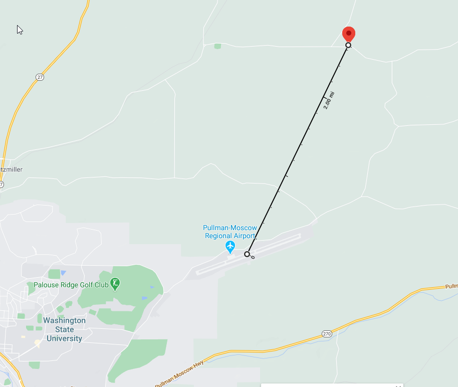
Figure 1: Estimated distance from weather reports to the crop fields. Distance is calculated using Google Maps
The second dataset comes from the USDA. This dataset consists of “hourly and daily measurements of volumetric water content, soil temperature, and bulk electrical conductivity, collected at 42 monitoring locations and 5 depths (30, 60, 90, 120, and 150 cm)” at a farm in Washington state 7. Mainly, the daily temperature and water content are the measurements of interest. There are multiple files that have data that corresponds to what plants are being grown in specific places, and the makeup of the soil at each sensor cite. This auxilary information could be used in later models once the base model has been completed. This data is in tab delimited files.
Within the data, there are GIS file types that can be imported into Google Maps desktop to visualize the locations of the sensors and other geographical information. Below is an example of the sensor locations plotted on the satellite image (see Figure 2).
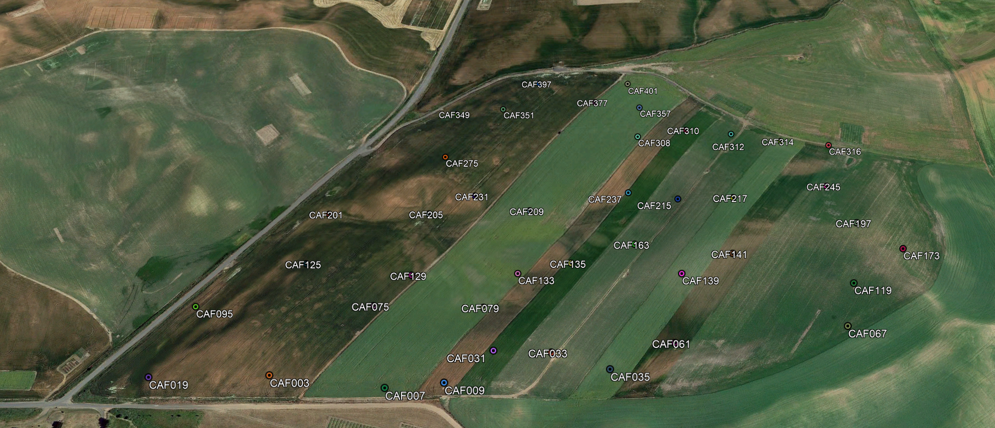
Figure 2: Location of sensors within the test field
4. Data Cleaning and Aggregation
The first step is to get the soil moisture data into a combined format, currently it is in one file per sensor, and there are 42 sensors. See the ml_pipeline.ipynb file to see how this was done, specifically the section titled “Data Processing”. After aggregation, some basic information can be checked about the data. For instance, there is quite a bit of NAs in the data. These NAs are just instances where there was no measurement on that day. There is about 45% NAs in the measurement columns. To further clean the data, any row that has only NAs for the measurements will be removed.
Next, the weather data needs some small adjustments. This is mostly in the form of removing columns that either are empty or have redundant data such as elevation, which is the same for every row.
Once the data is sufficiently clean, some choices have to be made on joining the data. The simplest route would be to join the weather measurements directly with the same day the soil measurement, however, the previous days weather is likely to also have an impact on the moisture. As evaluated in section 2 above, it is believed that the prior 16 days weather data is what is needed for a good prediction.
5. Pipeline for Preprocessing
Before feeding the data through a machine learning algorithm, the data needs to be manipulated in such a way that it is ready to be directly fed into an algorithm. This includes joining the two data sets, feature engineering, and other tasks that prepare the data. This will need to be done every time a new dataset is being used, so this must be built in a repeatable way. The machine learning library scikit-learn incorporates something called “pipelines” that can allow processed to be sequentially done to a dataframe. For purposes of this project two pipelines will be built, one will be used for feature engineering and joining the data, the other will be used to handle preparation of numerical, categorical, and date data. See sections: “Data Processing Pipeline” in ml_pipeline.ipynb.
5.1 Loading and Joining Data
This is the first step of the entire pipeline. This is where both the weather, and the soil moisture data are read in from csv files in their raw format. The soil moisture data is found in many different files, and these all need to be combined. After combining the files, any lines that are full of NAs for the measurements are dropped. Next the weather data is loaded in. Both files have a date field which is the field they will be joined on. To make things consistent, both of these fields need to set be date format.
When it comes to joining the data, each row should include the moisture content at various depths, as well as the weather information from the past ten days. While this creates a great deal of redundant data, the data is small enough that this is not an issue. Experiments will be done to evaluate just how many days of prior weather data are needed to form accurate results, while trying to minimize the number of the days.
5.2 Feature Engineering
Currently only two features are added, the first is a boolean flag that says whether it rained or not on a certain day. The thought behind this is, that for some days prior to the current measurement, the amount of rain might be needed, but for other days, such as 10 days prior, it might be more important to just know if there was rain or not. This feature is engineered within the pipeline.
The next feature is a categorical feature that is the month of the year. It isn’t very import to know the exact date of a measurement, but the month might be helpful in a model. This simplifies the model by not using date as a predictor, while still being able to capture this potentially important feature.
An excerpt of the code used to create these two features, this comes from ml_pipeline.ipynb.
soil['Month'] = pd.DatetimeIndex(soil['Date']).month

for i in range(17):
    col_name = 'PRCP_' + str(i)
    rain_y_n_name = 'RAIN_Y_N_' + str(i)
    X[rain_y_n_name] = np.nan
    X[rain_y_n_name].loc[X[col_name] > 0] = 1
    X[rain_y_n_name].loc[X[col_name] == 0] = 0
    X[rain_y_n_name] = X[rain_y_n_name].astype('object')
5.3 Generic Pipeline
After doing operations that are specific to the current dataset, some built in processors from sklearn are used to make sure the data can be used in a machine learning model. This means that for numerical data types, the pipeline will fill in missing values with 0 instead of leaving them as NaN. Also, the various numerical fields must be standardized, this is important for models such as linear regression so one large variable isn’t dominating the model.
As far as text and categorical features, the imputer will be used to fill in missing data as well. Then a process called one hot encoding will be used to handle the categorical variables so that they can be read into sklearns estimators. Lastly, these two main processes will be put together to make a single pipeline step. Then this pipeline step will be added to a regressor of some sort to create the entire process.
6. Multiple Models for Multiple Soil Depths
There are a few different approaches for modeling for this particular problem. The issue is that we have multiple things we would like to predict with the same predictors. It is unlikely that the model that predicts for a depth of 30 cm, would accurately predict for a depth of 150 cm. In order to adjust the models, a separate model will be created for each depth, with that said, the predictors are all the same for each depth, but the trained output is different. To accomplish this, five different datasets were constructed, each one representing a depth. All rows in which the predicted value is not available for that depth were pruned from the dataset.
In each experiment, there will be 5 different models created. Initially, these 5 models will use the same hyper-parameters for all the depths. It might turn out that all the models will need the same hyper-parameters, or each soil depth could be different. This will be examined through experimentation.
7. Splitting Data into Train and Test
In order to test any model created, there must be a split between test and training data. This is done by using a function in sklearn. In this case, there are about 76k rows in the data set. For the training data, 80% of the total data will be used, or about 60.8k records. The split is done after shuffling the rows so that it does not just pick the top 80% every time. Lastly the data is split using a stratified method. As we want to have models that take the specific area of the field into account, that means that we need to have the different areas of the field represented equally in both the training and testing dataset. This means that if 10% of the data came from sensor CAF0003, then roughly 10% of the training data will come from CAF0003 as well as 10% of the test data will be from this location.
8. Preliminary Analysis and EDA
Before building a machine learning model, it is important to get a general idea of how the data looks, to see if any insights can be made right away. The actual visualizations were built using a python package called Altair. This created the visualizations well, but the actual notebook that would contain these images was too large to include in their entirety.
The first two visualizations (viz_1, viz_2) are grids that show the entire distribution of measurements across each sensor. The first grid is the volume of water at 30 cm, and the second grid is the water volume at 150 cm. Each chart could be looked at and examined on it’s own, but what is most important to note is the variability of the measures from location to location. These different sensors are not that far away, but show that different areas of the farm do retain water in different ways. See Figure 3 for a small section of the grid from the visualization on the sensors at 30cm.
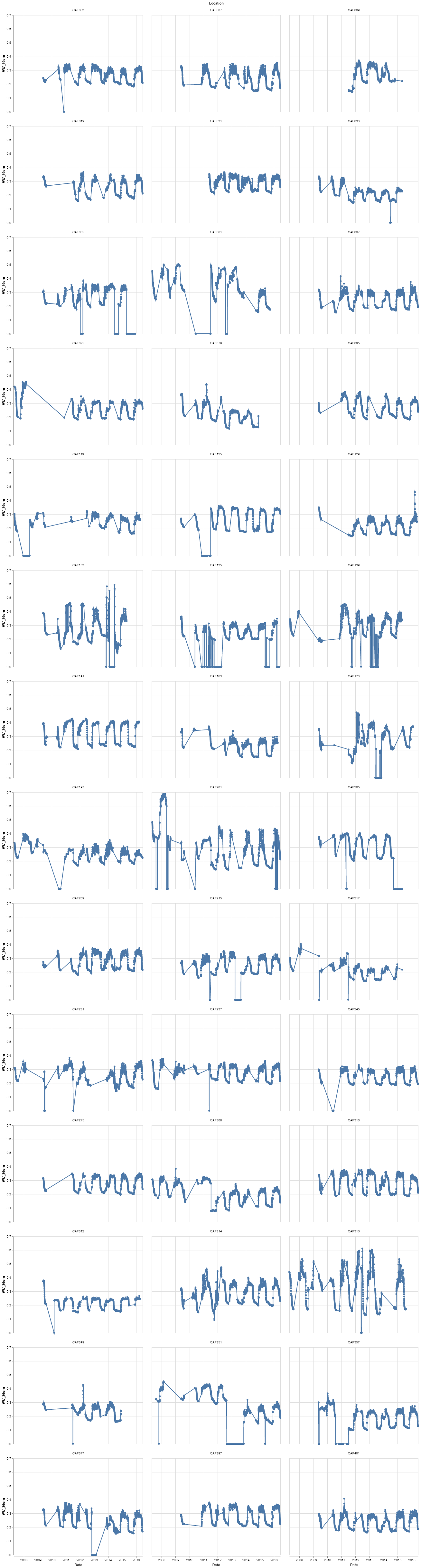
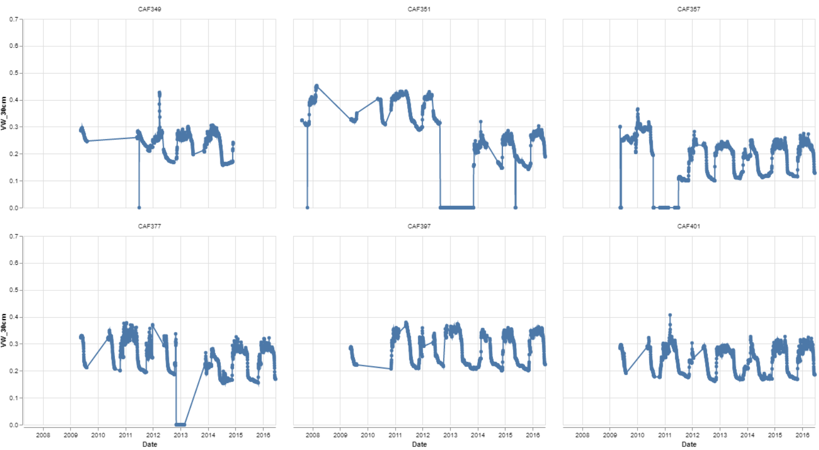
Figure 3: Six locations soil moisture level over time at 30 cm depth
The third and fourth grid shows the temperature at 150 cm, the results are what would logically be expected. The different sensors do not show much variance from location to location.
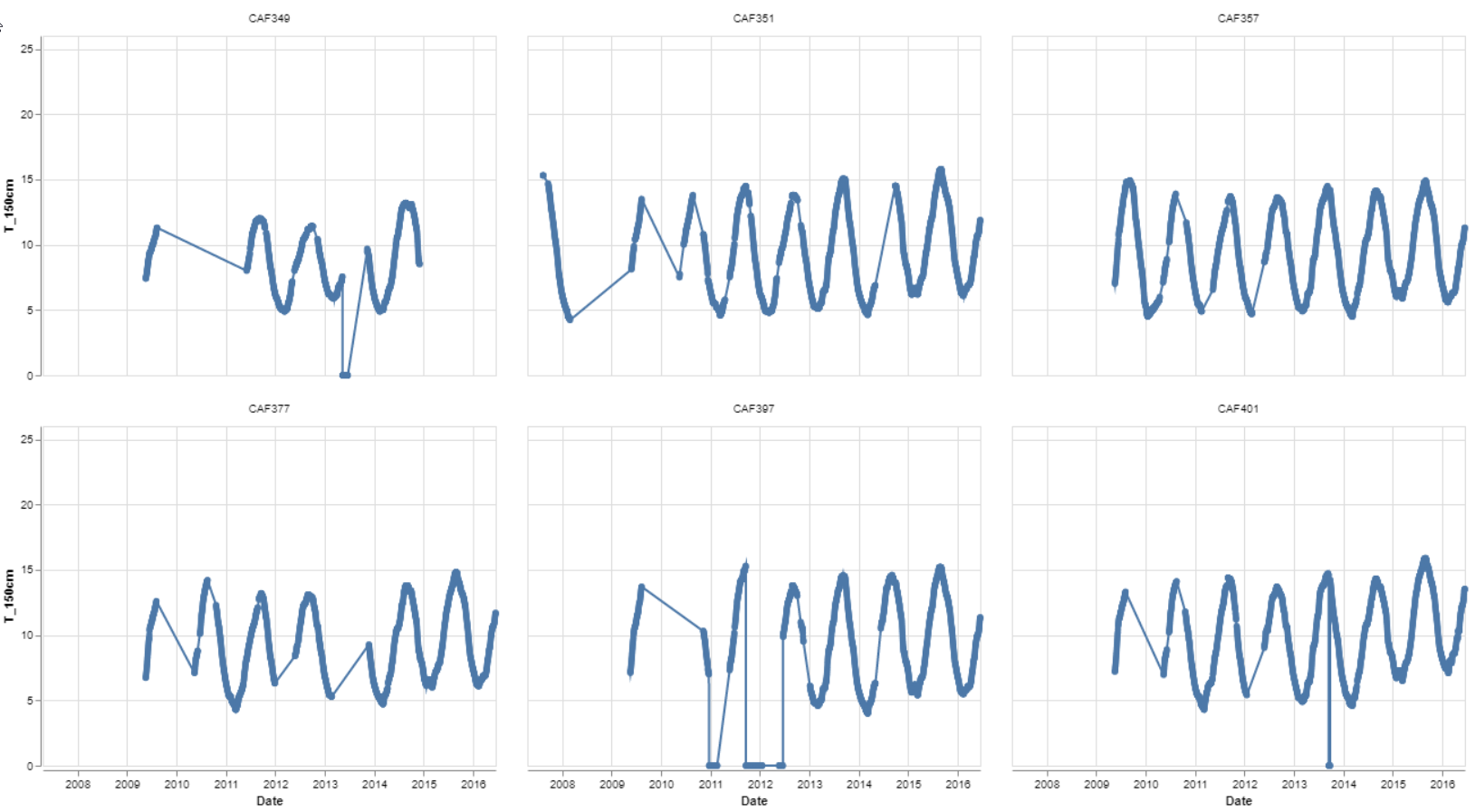
Figure 4: Six locations soil temperature over time at 150 cm depth
9. Initial Model Testing (Regressor)
Once the pipelines were setup, the first model could be tested for accuracy. As the output data is continuous in nature, the easiest machine learning algorithm to test to make sure everything is correct, was a linear regression model. It seems fairly likely that a linear regression model would do rather well with this data. The weather is the driving factor in soil moisture in a non-irrigated field, so this test is a litmus test to make sure that the data is good and provide a baseline measurement for future models. The experiment log below shows the returned values from the test that was run. Over the course of experimentation, a log such as this will be kept.
The results are as follows:
| Experiment | Depth | Fit_Time | Pred_Time | r2_score |
|---|---|---|---|---|
| First Linear Reg | 30cm | 2.029387 | 0.169824 | 9.16E-01 |
| First Linear Reg | 60cm | 2.002373 | 0.17377 | -1.42E+15 |
| First Linear Reg | 90cm | 2.080393 | 0.162992 | 9.49E-01 |
| First Linear Reg | 120cm | 2.299457 | 0.18056 | 9.46E-01 |
| First Linear Reg | 150cm | 2.573193 | 0.186042 | 9.43E-01 |
Figure 5: Baseline experiment results
These results show that the data is pretty well correlated and that there is reason to believe that we could predict soil moisture from weather alone. Although an r^2 of around 0.916-0.949 are pretty good, with such highly related predictors, there is definitely room for model improvement. Also for a depth of 60 cm, something is not predicting correctly and is resulting in a small negative r^2
10. Classifier vs. Regressor
While the output is continuous, there is an argument to use a categorical classifier model. For a specific plant, an optimal moisture range could be studied. For examples sake, the range could be 0.2-0.4 units. Then it would not matter if the soil is 0.2 or 0.3, both would be in the acceptable range. With this in mind, certain levels could be created to alert the farmer of which category they could be experiencing. For example there might be five levels: too dry, acceptable dryness, optimal, acceptable wetness, and too wet. The training data could be adjusted to fit into these categories.
Code to create a categorical variable for each of the depth measurements can be found in the section “Make Classifier Label” in the file: ml_pipeline.ipynb.
In the end, the decision to not use classifier methods was made. After using a regressor, the output could be converted to a categorical feature if the user or application so desired this. As our output is continuous in nature, precision would be lost.
11. Various Other Linear Regression Model Experiments
The next set of experiments came up with the results in the following table. This was a test to see if baseline Lasso or Ridge Regression would improve on the basic linear regression model. Results and code for this portion can be found in ml_pipeline.ipynb under the “Linear Regression Tests” section.
| Experiment | Depth | Fit_Time | Pred_Time | r2_score |
|---|---|---|---|---|
| Ridge Reg, Alpha = 1 | 30cm | 1.321553 | 0.173714 | 0.916211 |
| Ridge Reg, Alpha = 1 | 60cm | 1.29167 | 0.187392 | 0.942757 |
| Ridge Reg, Alpha = 1 | 90cm | 1.393526 | 0.197152 | 0.94879 |
| Ridge Reg, Alpha = 1 | 120cm | 1.307926 | 0.176656 | 0.946032 |
| Ridge Reg, Alpha = 1 | 150cm | 1.33738 | 0.179585 | 0.94332 |
| Lasso Reg, Alpha = 1 | 30cm | 1.45102 | 0.170752 | -0.00018 |
| Lasso Reg, Alpha = 1 | 60cm | 1.419546 | 0.174177 | -4.6E-05 |
| Lasso Reg, Alpha = 1 | 90cm | 1.4632 | 0.176657 | -5.7E-06 |
| Lasso Reg, Alpha = 1 | 120cm | 1.553091 | 0.182349 | -1.1E-06 |
| Lasso Reg, Alpha = 1 | 150cm | 1.437419 | 0.163967 | -0.00018 |
| Ridge Reg - GSCV | 30cm | 3.914718 | 0.203007 | 0.916235 |
| Ridge Reg - GSCV | 60cm | 3.726651 | 0.172752 | 0.942757 |
| Ridge Reg - GSCV | 90cm | 4.135154 | 0.200589 | 0.948796 |
| Ridge Reg - GSCV | 120cm | 4.03203 | 0.193512 | 0.946032 |
| Ridge Reg - GSCV | 150cm | 4.361977 | 0.191296 | 0.943328 |
Figure 6: Further Linear Regression Experiment Results
For the first two experiments, an alpha of 1 was used for both ridge and lasso regression. The third experiment used a special regressor that uses cross validation to try to find the best alpha value and then fit the model based on that. The best alpha value seemed to not have much effect at all on the results. Still the ridge regression so far was the best performing model.
12. Other Models
While there were great results in the different linear regression models, other models should be evaluated to make sure that something is not missed. Three models were chosen to check, Stochastic Gradient Descent, Support Vector Machine, and Random Forest. All of these models were tested with default parameters and their results are shown below in Figure 7, and the code can be found in the section called “Other Regressors Tests”.
| Experiment | Depth | Fit_Time | Pred_Time | r2_score |
|---|---|---|---|---|
| Random Forest | 30cm | 60.06952 | 0.250543 | 0.977118 |
| Random Forest | 60cm | 62.17435 | 0.216641 | 0.989113 |
| Random Forest | 90cm | 62.29475 | 0.243051 | 0.99158 |
| Random Forest | 120cm | 64.48227 | 0.256666 | 0.991274 |
| Random Forest | 150cm | 68.47001 | 0.240149 | 0.991748 |
| SVM | 30cm | 38.83822 | 5.712513 | 0.676934 |
| SVM | 60cm | 106.2816 | 7.897556 | 0.766008 |
| SVM | 90cm | 102.9438 | 7.763206 | 0.788833 |
| SVM | 120cm | 79.76476 | 6.985236 | 0.760895 |
| SVM | 150cm | 96.46352 | 7.548365 | 0.760936 |
| SGD | 30cm | 1.382992 | 0.171777 | 0.89019 |
| SGD | 60cm | 1.392753 | 0.15128 | 0.931394 |
| SGD | 90cm | 1.399587 | 0.142493 | 0.941092 |
| SGD | 120cm | 1.438626 | 0.150302 | 0.936692 |
| SGD | 150cm | 1.403488 | 0.14933 | 0.92957 |
Figure 7: Further Linear Regression Experiment Results
The random forest regressor performed amazingly in predicting the soil moisture. While the lower depths of soil did perform better than the depth of 30 cm. As random forests performed so well out of the box, some attempts were made to tune the hyperparameters, but most experiments turned out to be computationally expensive.
13. Conclusion
The end results of all experimentation was a process in which two datasets could be joined and fed into a model to predict the soil moisture with great accuracy, an r^2 score of between 0.977 and 0.991 depending on the depth using a Random Forest Regressor with default settings. This process could be a repeatable process in which a farmer contracts a company to gather training data on their land specifically for a growing season. As the collection of the sensor data could be cumbersome and expensive to deal with as a farmer, so this is an alternative that is cheaper and still gives nearly the same results as having sensors constantly running. Alternatively, this process could be a subprocess in a larger suite of software that farmers could use for predictive analysis or even to have data on soil moisture from a grow season to use in post season analysis of their crop produced. As long as large scale AI programs are still expensive and cumbersome for farmers to deal with, there will be a low rate of adoption. This project has shown that a solution for large scale soil moisture prediction software could be done with relatively low computational cost.
14. Acknowledgements
The author would like to thank Dr. Gregor Von Laszewski, Dr. Geoffrey Fox, and the associate instructors in the FA20-BL-ENGR-E534-11530: Big Data Applications course (offered in the Fall 2020 semester at Indiana University, Bloomington) for their continued assistance and suggestions with regard to exploring this idea and also for their aid with preparing the various drafts of this article.
15. References
-
O. Denmead and R. Shaw, “The Effects of Soil Moisture Stress at Different Stages of Growth on the Development and Yield of Corn 1”, Agronomy Journal, vol. 52, no. 5, pp. 272-274, 1960. Available: 10.2134/agronj1960.00021962005200050010x. ↩︎
-
K. Shang, S. Wang, Y. Ma, Z. Zhou, J. Wang, H. Liu and Y. Wang, “A scheme for calculating soil moisture content by using routine weather data”, Atmospheric Chemistry and Physics, vol. 7, no. 19, pp. 5197-5206, 2007 [Online]. Available: https://hal.archives-ouvertes.fr/hal-00302825/document ↩︎
-
W. Capehart and T. Carlson, “Estimating near-surface soil moisture availability using a meteorologically driven soil-water profile model”, Journal of Hydrology, vol. 160, no. 1-4, pp. 1-20, 1994 [Online]. Available: https://tinyurl.com/yxjyuy5x ↩︎
-
F. Pan, C. Peters-Lidard and M. Sale, “An analytical method for predicting surface soil moisture from rainfall observations”, Water Resources Research, vol. 39, no. 11, 2003 [Online]. Available: https://agupubs.onlinelibrary.wiley.com/doi/pdf/10.1029/2003WR002142. [Accessed: 08- Nov- 2020] ↩︎
-
C. Gasch, D. Brown, C. Campbell, D. Cobos, E. Brooks, M. Chahal and M. Poggio, “A Field-Scale Sensor Network Data Set for Monitoring and Modeling the Spatial and Temporal Variation of Soil Water Content in a Dryland Agricultural Field”, Water Resources Research, vol. 53, no. 12, pp. 10878-10887, 2017 [Online]. Available: https://agupubs.onlinelibrary.wiley.com/doi/full/10.1002/2017WR021307. [Accessed: 08- Nov- 2020] ↩︎
-
N. (NCEI), “Climate Data Online (CDO) - The National Climatic Data Center’s (NCDC) Climate Data Online (CDO) provides free access to NCDC’s archive of historical weather and climate data in addition to station history information. | National Climatic Data Center (NCDC)”, Ncdc.noaa.gov, 2020. [Online]. Available: https://www.ncdc.noaa.gov/cdo-web/. [Accessed: 19- Oct- 2020]. ↩︎
-
“Data from: A field-scale sensor network data set for monitoring and modeling the spatial and temporal variation of soil moisture in a dryland agricultural field”, USDA: Ag Data Commons, 2020. [Online]. Available: https://data.nal.usda.gov/dataset/data-field-scale-sensor-network-data-set-monitoring-and-modeling-spatial-and-temporal-variation-soil-moisture-dryland-agricultural-field. [Accessed: 19- Oct- 2020]. ↩︎