Project: Forecasting Natural Gas Demand/Supply

Status: final, Type: Project

Baekeun Park, sp21-599-356, Edit

• Code:
  • Forecasting_NG_Demand_Supply.ipynb

Keywords: Natural Gas, supply, forecasting, South Korea, MLP with LSTM, Tensorflow, various dataset.

1. Introduction

South Korea relies on imports for 92.8 percent of its energy resources as of the first half of 2020 ¹. Among the energy resources, the Korea Gas Corporation(KOGAS) imports Liquified Natural Gas(LNG) from around the world and supplies it to power generation plants, gas-utility companies, and city gas companies throughout the country ². It produces and supplies NG in order to ensure a stable gas supply for the nation. Moreover, it operates LNG storage tanks at LNG acquisition bases, storing LNG during the season when city gas demand is low and replenish LNG during winter when demand is higher than supply ³.

The wholesale charges consist of raw material costs (LNG introduction and incidental costs) and gas supply costs ⁴. Therefore, the forecasting NG demand/supply will help establish an optimized mid-to-long-term plan for the introduction of LNG and stable NG supply and economic effects.

The factors which influence NG demand include weather, economic conditions, and petroleum prices. The winter weather strongly influences NG demand, and the hot summer weather can increase electric power demand for NG. In addition, some large-volume fuel consumers such as power plants and iron, steel, and paper mills can switch between NG, coal, and petroleum, depending on the cost of each fuel ⁵.

Therefore, some indicators related to weather, economic conditions, and the price of other energy resources can be used for this project.

2. Related Work

Khotanzad and Elragal (1999) proposed a two-stage system with the first stage containing a combination of artificial neural network(ANN) for prediction of daily NG consumption ⁶, and Khotanzad et al. (2000) combined eight different algorithms to improve the performance of forecasters ⁷. Mustafa Akpinar et al. (2016) used daily NG consumption data to forecast the NG demand by ABC-based ANN ⁸. Also, Athanasios Anagnostis et al. (2019) conducted daily NG demand prediction by a comparative analysis between ANN and LSTM ⁹. Unlike those methods, MLP with LSTM is applied for this project, and external factors affecting NG demand are changed and compared.

3. Datasets

As described, weather datasets like temperature and precipitation, price datasets of other energy resources like crude oil and coal, and economic indicators like exchange rate are used in this project for forecasting NG demand and supply.

There is an NG supply dataset ¹⁰ from a public data portal in South Korea. It includes four years from 2016 to 2019 of regional monthly NG supply in the nine different cities of South Korea. In addition, climate data such as temperature and precipitation ¹¹ for the same period can be obtained from the Korea Meteorological Administration. Similarly, data on the price of four types of crude oil ¹² and various types of coal price datasets per month ¹³ are also available through corresponding agencies. Finally, the Won-Dollar exchange rate dataset ¹⁴ with the same period is used.

As mentioned above, each dataset has monthly information and also has average values instead of the NG supply dataset. It is regionally separated or combined according to the test scenario. For example, the NG supply dataset has nine different cities. One column of cities is split from the original dataset and merged with another regional dataset like temperature or precipitation. On the other hand, each regional value’s summation is utilized in a scenario where a national dataset is needed.

The dataset is applied differently for each scenario. In scenario one, all datasets such as crude oil price, coal price, exchange rate, and regional temperature and precipitation are merged with regional dataset, especially Seoul. For scenario two, all climate datasets are used with the regional dataset. Only temperature dataset is utilized with regional dataset in scenario three. In addition, in scenario four, all cases are the same as in scenario one, but the timesteps are changed to two months. Finally, the national dataset is used for scenario five.

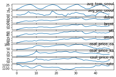
Figure 1: External factors affecting natural gas

4. Methodology

4.1. Min-Max scaling

In this project, all datasets are rescaled between 0 and 1 by Min-Max scaling, one of the most common normalization methods. If there is a feature with anonymous data, The maximum value(max(x)) of data is converted to 1, and the minimum value(min(x)) of data is converted to 0. The other values between the maximum value and the minimum value get converted to x', between 0 and 1.

4.2. Training

For forecasting the NG supply amount from the time series dataset, MLP with LSTM network model is designed by using Tensorflow. The first and second LSTM layers have 100 units, and a total of 3 layers of MLP follow it. Each MLP layer has 100 neurons instead of the final layer, where its neuron is 1. In addition, dropout was designated to prevent overfitting of data, the Adam is used as an optimizer, and the Rectified Linear Unit(ReLU) as an activation function.

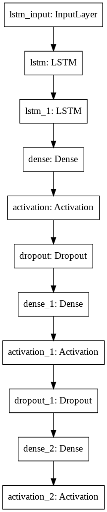
Figure 2: Structure of network model

4.3. Evaluation

Mean Absolute Error(MAE) and Root Mean Squared Error(RMSE) are applied for this time series dataset to evaluate this network model. The MAE measures the average magnitude of the errors and is presented by the formula as following, where n is the number of errors, is the true value, and is the predicted value.

Also, The RMSE is used for observing the differences between the actual dataset and prediction values. The following is the formula of RMSE, and each value of this is the same for MAE.

4.4. Prediction

Since the datasets used for the training process are normalized between 0 and 1, they get converted to a range of the ground truth values again. From these rescaled datasets, it is possible to obtain the RMSE and compare the differences between the actual value and the predicted value.

5. Result

In all scenarios, main variables such as dropout, learning rate, and epochs are fixed under the same conditions and are 0.1, 0.0005, and 100 in order. In scenarios one, two, three, and five, the training set is applied as twelve months, and in scenario four, next month’s prediction comes from the previous two months dataset. For comparative analysis, the results are obtained by changing the size of the training set from twelve months to twenty-four months, and the effect is described. Each scenario shows individual results and is comprehensively compared at the end of this part.

5.1 Scenario one(regional dataset)

The final MAE of the train set is around 0.05, and the one of the test set is around 0.19. Also, the RMSE between actual data and predicted data is around 227018. The predictive graph tends to deviate a lot at the beginning of the part, but it shows a relatively similar shape at the end of the graph.

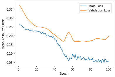
Figure 3: Loss for scenario one

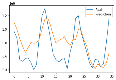
Figure 4: Prediction results for scenario one

5.2 Scenario two(regional climate dataset)

The final MAE of the train set is around 0.10, and the one of the test set is around 0.14. Also, the RMSE is around 185205. Although the predictive graph still differs compared to the actual graph, it shows similar trends in shape.

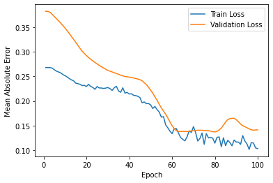
Figure 5: Loss for scenario two

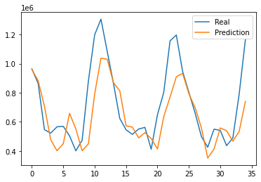
Figure 6: Prediction results for scenario two

5.3 Scenario three(regional temperature dataset)

The final MAE of the train set is around 0.13, and the one of the test set is around 0.14. Also, the RMSE is around 207585. While the tendency to follow high and low seems similar, but changes in the middle seem to be misleading.

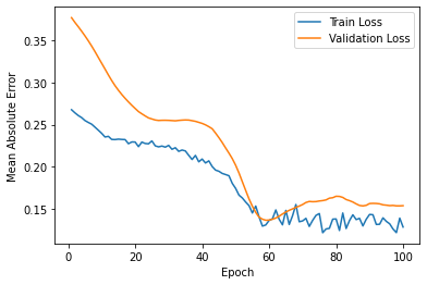
Figure 7: Loss for scenario three

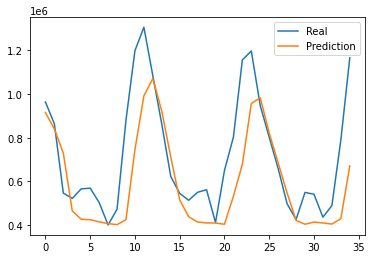
Figure 8: Prediction results for scenario three

5.4 Scenario four(applying timesteps)

The final MAE of the train set is around 0.06, and the one of the test set is around 0.30. Also, the RMSE is around 340843. Out of all scenarios, the predictive graph shows to have the most differences. However, in the last part, there is a somewhat akin tendency.

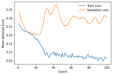
Figure 9: Loss for scenario four

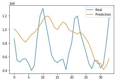
Figure 10: Prediction results for scenario four

5.5 Scenario five(national dataset)

The final MAE of the train set is around 0.03 and the one of test set is around 0.14. Also, the RMSE between real data and predicted data is around 587340. Tremendous RMSE value results, but direct comparisons are not possible because the baseline volume is different from other scenarios. Although the predictive graph shows discrepancy, it tends to be similar to the results in scenario two.

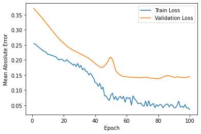
Figure 11: Loss for scenario five

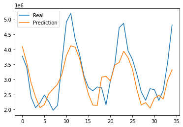
Figure 12: Prediction results for scenario five

5.6 Overall results

Out of the five scenarios in total, the second and third have smaller RMSE than others, and the graphs also show relatively similar results. The first and fourth show differences in the beginning and similar trends in the last part. However, it is noteworthy that the gap at the beginning of them is very large, but it tends to shrink together at the point of decline and stretch together at the point of increase.

In the first and fifth scenarios, all data are identical except that they differ in regional scale in temperature and precipitation. It is also the same that twelve months of data are used as the training set. From the subtle differences in the shape of the resulting graph, it can be seen that the national average data cannot represent the situation in a particular region, and the amount of NG supply differs depending on the circumstances in the region.

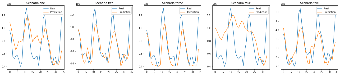
Figure 13: Total prediction results: 12 months training set

After changing the training set from twelve months to twenty-four months, the results are more clearly visible. The second and third prediction graphs have a more similar shape and the RMSE value decreases than the previous setting. The results of other scenarios show that the overall shape has improved; contrarily, the shape of the rapidly changing middle part is better in the previous condition.

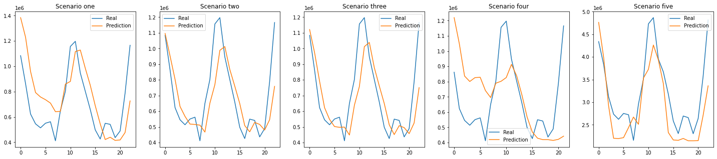
Figure 14: Total prediction results: 24 months training set

6. Benchmarks

For a benchmark, the Cloudmesh StopWatch and Benchmark ¹⁵ is used to measure the program’s performance. The time spent on data load, data preprocessing, network model compile, training, and the prediction was separately measured, and the overall time for execution of all scenarios is around 77 seconds. It can be seen that The training time for the fourth scenario is the longest, and the one for the fifth scenario is the shortest.

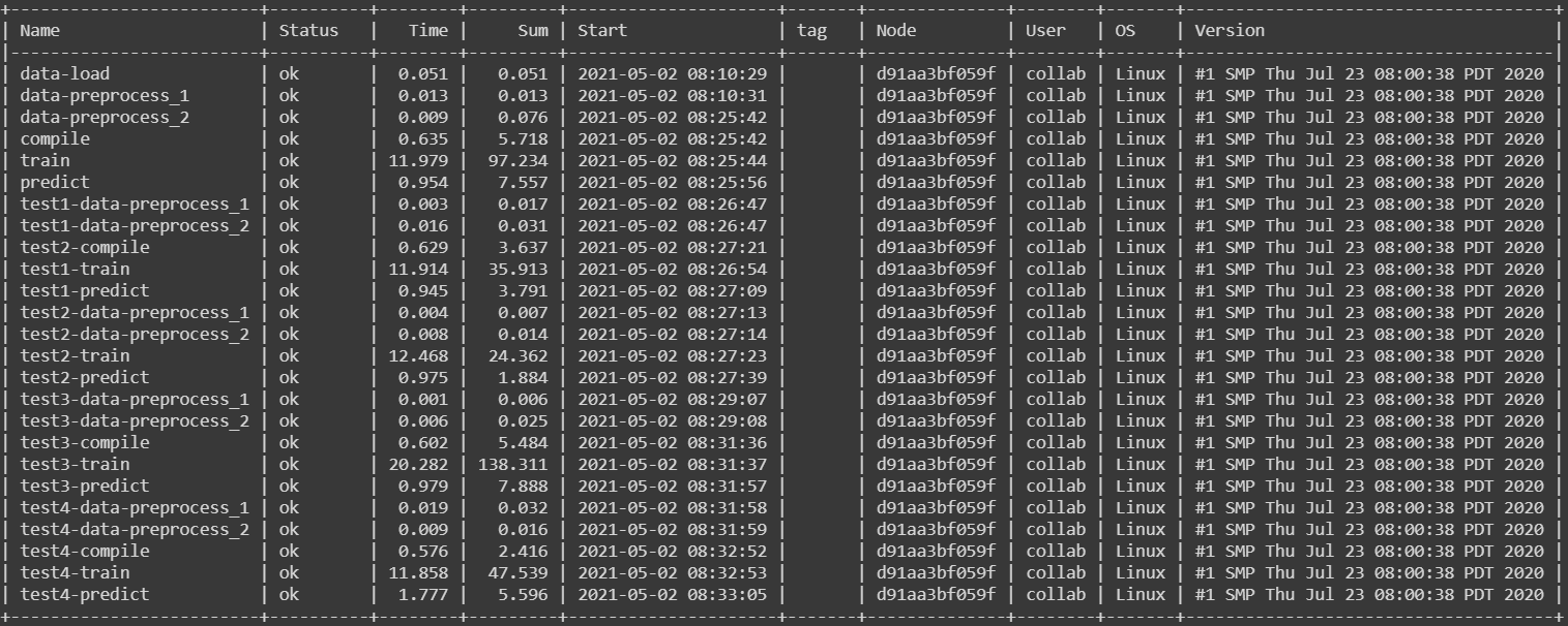
Figure 15: Benchmarks

7. Conclusion

From the results of this project, it can be seen that simplifying factors that have a significant impact shows better efficiency than combining various factors. For example, NG consumption tends to increase for heating in cold weather. In addition, there is much precipitation in warm or hot weather; on the contrary, there is relatively little precipitation in the cold weather. It can be seen that these seasonal elements show relatively high consistency for affecting prediction when those are used as training datasets. Also, the predictions are derived more effectively when the seasonal datasets are combined.

However, in training set with a duration of twelve months, the last part of the scenario tends to match the actual data despite using the dataset combined with various factors that appears to be seasonally unrelated. Furthermore, when the training set is doubled on the same dataset, it can be seen that the differences between the actual and prediction graph are decreased than the result of a smaller training set. Based on this, it can be expected that the results could vary if a large amount of dataset with a more extended period is used and the ratio of the training set is appropriately adjusted.

South Korea imports a large amount of its energy resources. Also, the plan for energy demand and supply is being made and operated through nation-led policies. Ironically, the government’s plan also shows a sharp change in direction with recent environmental issues, and the volatility of demand in the energy market is increasing than before. Therefore, methodologies for accurate forecasting of energy demand will need to be complemented and developed constantly to prepare for and overcome this variability.

In this project, Forecasting NG demand and supply was carried out using various data factors such as weather and price that is relatively easily obtained than the datasets which are complex economic indicators or classified as confidential. Nevertheless, state-of-the-art deep learning methods show that it has the flexibility and potential to forecast NG demand through the tendency of the results that indicate a relatively consistent with the actual data. From this point of view, it is thought that the research on NG in South Korea should be conducted in an advanced form by utilizing various data and more specialized analysis.

8. Acknowledgments

The author would like to thank Dr. Gregor von Laszewski for his invaluable feedback, continued assistance, and suggestions on this paper, and Dr. Geoffrey Fox for sharing his expertise in Deep Learning and Artificial Intelligence applications throughout this Deep Learning Application: AI-First Engineering course offered in the Spring 2021 semester at Indiana University, Bloomington.

9. Source code

The source code for all experiments and results can be found here as ipynb link and as pdf link.

10. References