Analysis of Various Machine Learning Classification Techniques in Detecting Heart Disease
18 minute read
![]()
![]() Status: final, Type: Project
Status: final, Type: Project
Ethan Nguyen, fa20-523-309, Edit
Abstract
As cardiovascular diseases are the number 1 cause of death in the United States, the study of the factors and early detection and treatment could improve quality of life and lifespans. From investigating how the variety of factors related to cardiovascular health relate to a general trend, it has resulted in general guidelines to reduce the risk of experiencing a cardiovascular disease. However, this is a rudimentary way of preventative care that allows for those who do not fall into these risk categories to fall through. By applying machine learning, one could develop a flexible solution to actively monitor, find trends, and flag patients at risk to be treated immediately. Solving not only the risk categories but has the potential to be expanded to annual checkup data revolutionizing health care.
Contents
Keywords: health, healthcare, cardiovascular disease, data analysis
1. Introduction
Since cardiovascular diseases are the number 1 cause of death in the United States, early prevention could help in extending one’s life span and possibly quality of life 1. Since there are cases where patients do not show any signs of cardiovascular trouble until an event occurs, having an algorithm predict from their medical history would help in picking up on early warning signs a physician may overlook. Or could also reveal additional risk factors and patterns for research on prevention and treatment. In turn this would be a great tool to apply in preventive care, which is the type of healthcare policy that focuses in diagnosing and preventing health issues that would otherwise require specialized treatment or is not treatable 2. This also has the potential to trickle down and increase the quality of life and lifespan of populations at a reduced cost as catching issues early most likely results in cheaper treatments 2.
This project will take a high-level overview of common, widely available classification algorithms and analyze their effectiveness for this specific use case. Notable ones include, Gaussian Naive Bayes, K-Nearest Neighbors, and Support Vector Machines. Additionally, two data sets that contain common features will be used to increase the training and test pool for evaluation. As well as to explore if additional feature types contribute to a better prediction. The goal of this project being a gateway to further research in data preprocessing, tuning, or development of specialized algorithms as well as further ideas on what data could be provided.
2. Datasets
- https://www.kaggle.com/johnsmith88/heart-disease-dataset
- https://www.kaggle.com/sulianova/cardiovascular-disease-dataset
The range of creation dates are 1988 and 2019 respectively with different features of which 4 are common between. This does bring up a small hiccup in preprocessing to consider. Namely the possibility of changing diet and culture trends resulting in significantly different trends/patterns within the same age group. As well as possible differences in measurement accuracy. However this large gap is within the scope of the project in exploring which features can help provide an accurate prediction.
This possible phenomenon may be of interest to explore closely if time allows. Whether a trend itself is even present or there is an overarching trend across different cultures and time periods. Or to consider if this difference is significant enough that the data from the various sets needs to be adjusted to normalize the ages to present day.
2.1 Dataset Cleaning
The datasets used have already been significantly cleaned from the raw data and has been provided as a csv file. These files were then imported into the python notebook as pandas dataframes for easy manipulation.
An initial check was made to ensure the integrity of the data matched the description from the source websites. Then some preprocessing was completed to normalize the common features between the datasets. These features were gender, age, and cholesterol levels. The first two adjustments were trivial in conversion however, in the case of cholesterol levels, the 2019 set is on a 1-3 scale while the 1988 dataset provided them as real measurements. A conversion of the 1988 dataset was done based on guidelines found online for the age range of the dataset 3.
2.2 Dataset Analysis
From this point on, the 1988 dataset will be referred to as dav_set and 2019 data set will be referred to as sav_set.
To provide further insight on what to expect and how a model would be applied, the population of the datasets was analysed first. As depicted in Figure 2.1 the population samples of both datasets of gender vs age show the majority of the data is centered around 60 years of age with a growing slope from 30 onwards.
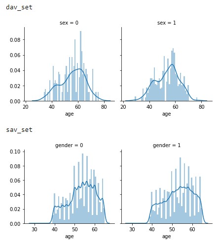
Figure 2.1: Age vs Gender distributions of the dav_set and sav_set.
This trend appears to signify that the datasets focused solely on an older population or general trend in society of not monitoring heart conditions as closely in the younger generation.
Moving on to Figure 2.2, we see an interesting trend with a significant growing trend in the sav_set in older population having more cardiovascular issues compared to the dav_set. While this cannot be seen in the dav_set. This may be caused by the additional life expectancy or a change in diet as noted in the introduction.
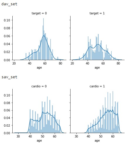
Figure 2.2: Age vs Target distributions of the dav_set and sav_set.
In Figure 2.3, the probability of having cardiovascular issues between the sets are interesting. In the dav_set the inequality of higher probability could be attributed to the larger female samples in the dataset. With the sav_set having a more equal probability between the genders.
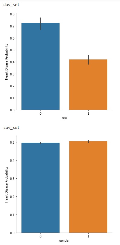
Figure 2.3: Gender vs Probability of cardiovascular issues of the dav_set and sav_set.
Finally, in Figure 2.4 is the probability vs cholesterol levels. This one is very interesting between the two datasets in terms of trend levels. With the dav_set having a higher risk at normal levels compared to the sav_set. This could be another hint of a societal change across the years or may in fact be due to the low sample size. Especially since the sav_set matches the general consensus of higher cholesterol levels increasing risk of cardiovascular issues 3.
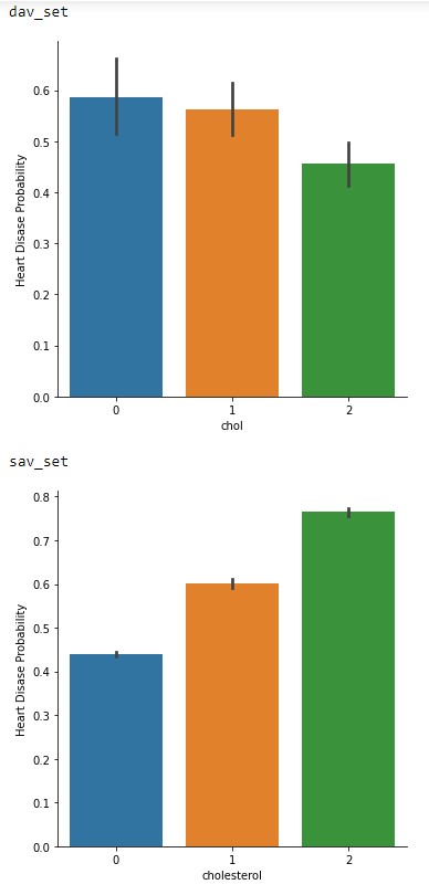
Figure 2.4: Cholesterol levels vs Probability of cardiovascular issues of the dav_set and sav_set.
To close out this initial analysis is the correlation map of each of the features. From Figure 2.5 and 2.6 it can be concluded that both of these datasets are viable to conduct machine learning as the correlation factor is below the recommended value of 0.8 4. Although we do see the signs of a low sample amount in the dav_set with a higher correlation factor compared to the sav_set.
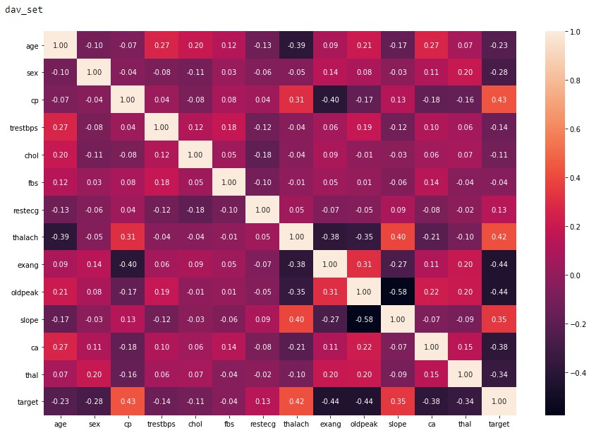
Figure 2.5: dav_set correlation matrix.

Figure 2.6: sav_set correlation matrix.
3. Machine Learning Algorithms and Implementation
With many machine learning algorithms already available and many more in development. Selecting the optimal one for an application can be a challenging balance since each algorithm has both its advantages and disadvantages. As mentioned in the introduction, we will explore applying the most common and established algorithms available to the public.
Starting off, is selecting a library from the most popular ones available. Namely Keras, Pytorch, Tensorflow, and Scikit-Learn. Upon further investigation it was determined that Scikit-Learn would be used for this project. The reason being Scikit-Learn is a great general machine learning library that also includes pre and post processing functions. While Keras, Pytorch, and Tensorflow are targeted for neural networks and other higher-level deep learning algorithms which are outside of the scope of this project at this time 5.
3.1 Scikit-Learn and Algorithm Types
Diving further into the Scikit-Learn library, its key strength appears to be the variety of algorithms available that are relatively easy to implement against a dataset. Of those available, they are classified under three different categories based on the approach each takes. They are as follows:
- Classification
- Applied to problems that require identifying the category an object belongs to.
- Regression
- For predicting or modeling continuous values.
- Clustering
- Grouping similar objects into groups.
For this project, we will be investigating the Classification and Clustering algorithms offered by the library due to the nature of our dataset. Since it is a binary answer, the continuous prediction capability of regression algorithms will not fair well. Compared to classification type algorithms which are well suited for determining binary and multi-class classification on datasets 6. Along with Clustering algorithms being capable of grouping unlabeled data which is one of the key problem points mentioned in the introduction 7.
3.2 Classification Algorithms
The following algorithms were determined to be candidates for this project based on the documentation available on the Scikit-learn for supervised learning 8.
3.2.1 Support Vector Machines
This algorithm was chosen because classification is one of the target types and has a decent list of advantages that appear to be applicable to this dataset 6.
- Effective in high dimensional spaces as well as if the number dimensions out number samples.
- Is very versatile.
3.2.2 K-Nearest Neighbors
This algorithm was selected due to being a non-parametric method that has been successful in classification applications 9. From the dataset analysis, it is appears that the decision boundary may be very irregular which is a strong point of this type of method.
3.2.3 Gaussian Naive Bayes
Is an implementation of the Naive Bayes theorem that has been targeted for classification. The advantages of this algorithm is its speed and requires a small training set compared to more advanced algorithms 10.
3.2.4 Decision Trees
This algorithm was chosen to investigate another non-parametric method to determine their efficacy against this dataset application. This algorithm also has some advantages over K-Nearest namely 11.
- Simple to interpret and visualize
- Requires little data preparation
- Handles numerical and categorical data instead of needing to normalize
- Can validate the model and is possible to audit from a liability standpoint.
3.3 Clustering Algorithms
The following algorithms were determined to be candidates for this project based on the table of clustering algorithms available on the Scikit-learn 7.
3.3.1 K-Means
The usecase for this algorithm is general purpose with even and low number of clusters 7. Of which the sav_set appears to have with the even distribution across most of the features.
3.3.2 Mean-shift
This algorithm was chosen for its strength in dealing with uneven cluster sizes and non-flat geometry 7. Though it is not easily scalable the application of our small dataset size might be of interest.
3.3.3 Spectral Clustering
As an inverse, this algorithm was chosen for its strength with fewer uneven clusters 7. In comparison to Mean-shift, this maybe the better algorithm for this application.
3.4 Implementation
The implementation of these algorithms were done under the direction of the documentation page for each respective algorithm. The jupyter notebook used for this project is available at https://github.com/cybertraining-dsc/fa20-523-309/blob/main/project/data_analysis/ml_algorithms.ipynb with each algorithm having a corresponding cell. A benchmarking library is also included to determine the efficiency of each algorithm in processing time. One thing of note is the lack of functions used for the classification compared to the clustering algorithms. The justification for this discrepancy is due to inexperience in creating optimal implementations as well as determining that not being implemented in a function would not have a significant impact on performance. Additionally, graphs representing the test data were included to help visualize the performance of the clustering algorithms utilizing example code from the documentation 12.
3.4.1 Dataset Preprocessing
Pre-processing of the cleaned datasets for the classification algorithms was done under guidance of the scikit learn documentation 13. Overall, each algorithm was trained and tested with the same split for each run. While the split data could have been passed directly to the algorithms, they were normalized further using the built-in fit_transform function for the best results possible.
Pre-processing of the cleaned datasets for the clustering algorithms was done under guidance of the scikit learn documentation 7. Compared to the classification algorithms, a dimensionality reduction was conducted using Principal component analysis (PCA). This step condenses the multiple features into a 2 feature array which the clustering algorithms were optimized for, increasing the odds for the best results possible. Another note is the dataset split was conducted during execution of the algorithm. Upon further investigation, it was determined that this does not have an effect on the ending results as the randomization was disabled due to setting the same random_state parameter for each call.
4. Results & Discussion
4.1 Algorithm Metrics
The metrics used to determine the viability of each of the algorithms are precision, recall, and f1-score. These are simple metrics based on the values from a confusion matrix which is a visualization of the False and True Positives and Negatives. Precision is essentially how accurate was the algorithm in classifying each data point. This however, is not a good metric to solely base performance as precision does not account for imbalanced distributions within a dataset 14.
This is where the recall metric comes in which is defined as how many samples were accurately classified by the algorithm. This is a more versatile metric as it can compensate for imbalanced datasets. While it may not be in our case as seen in the dataset analysis where we have a relatively balanced ratio. It still gives great insight on the performance for our application.
Finally is the f1-score which is the harmonic mean of the precision and recall metric 14. This will be the key metric we will mainly focus on as it strikes a good balance between the two more primitive metrics. Since one may think in medical applications one would want to maximize recall, it is at the cost of precision which ends up in more false predictions which is essentially an overfitting scenario 14. Something that reduces the viability of the model to the application especially since we have a relatively balanced dataset, more customized weighting is not as necessary.
The metrics for each algorithm implementation are as follows. The training time metric is provided by the cloudmesh.common benchmark library 15.
4.1.1 Support Vector Machines
Table 4.1: dav_set metrics
| Precision | Recall | f1-score | |
|---|---|---|---|
| No Disease | 0.99 | 0.94 | 0.96 |
| Has Disease | 0.95 | 0.99 | 0.97 |
| Training Time | 0.038 sec |
Table 4.2: sav_set metrics
| Precision | Recall | f1-score | |
|---|---|---|---|
| No Disease | 0.99 | 0.94 | 0.96 |
| Has Disease | 0.95 | 0.99 | 0.97 |
| Training Time | 167.897 sec |
4.1.2 K-Nearest Neighbors
Table 4.3: dav_set metrics
| Precision | Recall | f1-score | |
|---|---|---|---|
| No Disease | 0.88 | 0.86 | 0.87 |
| Has Disease | 0.87 | 0.90 | 0.88 |
| Training Time | 0.025 sec |
Table 4.4: sav_set metrics
| Precision | Recall | f1-score | |
|---|---|---|---|
| No Disease | 0.62 | 0.74 | 0.67 |
| Has Disease | 0.67 | 0.54 | 0.60 |
| Training Time | 10.116 sec |
4.1.3 Gaussian Naive Bayes
Table 4.5: dav_set metrics
| Precision | Recall | f1-score | |
|---|---|---|---|
| No Disease | 0.88 | 0.81 | 0.84 |
| Has Disease | 0.83 | 0.90 | 0.86 |
| Training Time | 0.011 sec |
Table 4.6: sav_set metrics
| Precision | Recall | f1-score | |
|---|---|---|---|
| No Disease | 0.56 | 0.90 | 0.69 |
| Has Disease | 0.72 | 0.28 | 0.40 |
| Training Time | 0.057 sec |
4.1.4 Decision Trees
Table 4.7: dav_set metrics
| Precision | Recall | f1-score | |
|---|---|---|---|
| No Disease | 0.92 | 0.97 | 0.95 |
| Has Disease | 0.97 | 0.93 | 0.95 |
| Training Time | 0.009 sec |
Table 4.8: sav_set metrics
| Precision | Recall | f1-score | |
|---|---|---|---|
| No Disease | 0.71 | 0.80 | 0.75 |
| Has Disease | 0.76 | 0.66 | 0.71 |
| Training Time | 0.272 sec |
4.1.5 K-Means
Figure 4.1: dav_set algorithm visualization. The axis have no corresponding unit due to the PCA operation.
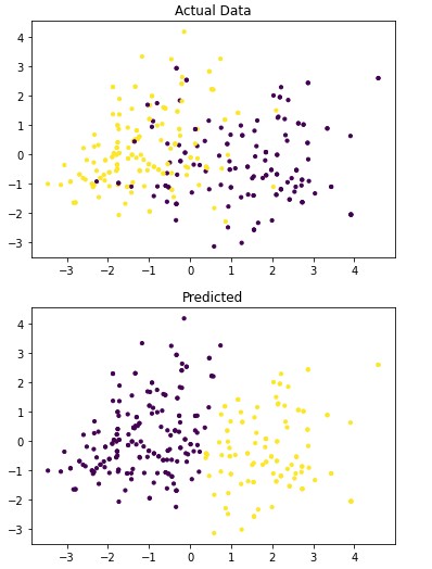
Table 4.9: dav_set metrics
| Precision | Recall | f1-score | |
|---|---|---|---|
| No Disease | 0.22 | 0.29 | 0.25 |
| Has Disease | 0.12 | 0.09 | 0.10 |
| Training Time | 0.376 sec |
Figure 4.2: sav_set algorithm visualization. The axis have no corresponding unit due to the PCA operation.
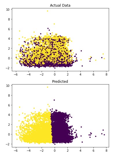
Table 4.10: sav_set metrics
| Precision | Recall | f1-score | |
|---|---|---|---|
| No Disease | 0.51 | 0.69 | 0.59 |
| Has Disease | 0.52 | 0.34 | 0.41 |
| Training Time | 1.429 sec |
4.1.6 Mean-shift
Figure 4.3: dav_set algorithm visualization. The axis have no corresponding unit due to the PCA operation.
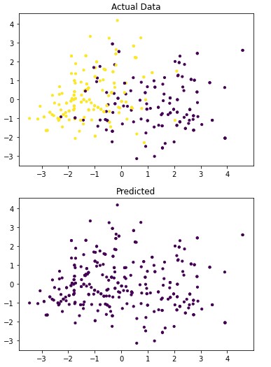
Table 4.11: dav_set metrics
| Precision | Recall | f1-score | |
|---|---|---|---|
| No Disease | 0.47 | 1.00 | 0.64 |
| Has Disease | 0.00 | 0.00 | 0.00 |
| Training Time | 0.461 sec |
Figure 4.4: sav_set algorithm visualization. The axis have no corresponding unit due to the PCA operation.
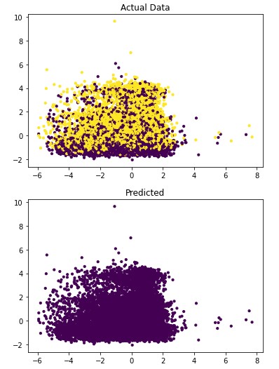
Table 4.12: sav_set metrics
| Precision | Recall | f1-score | |
|---|---|---|---|
| No Disease | 0.50 | 1.00 | 0.67 |
| Has Disease | 0.00 | 0.00 | 0.00 |
| Training Time | 193.93 sec |
4.1.7 Spectral Clustering
Figure 4.5: dav_set algorithm visualization. The axis have no corresponding unit due to the PCA operation.
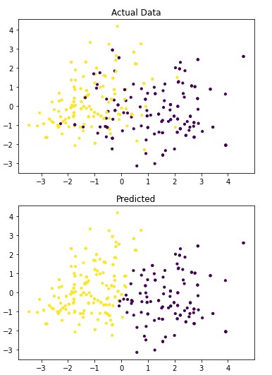
Table 4.13: dav_set metrics
| Precision | Recall | f1-score | |
|---|---|---|---|
| No Disease | 0.86 | 0.74 | 0.79 |
| Has Disease | 0.79 | 0.89 | 0.84 |
| Training Time | 0.628 sec |
Figure 4.6: sav_set algorithm visualization. The axis have no corresponding unit due to the PCA operation.
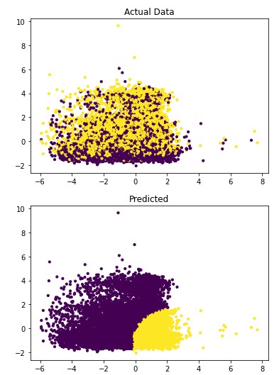
Table 4.14: sav_set metrics
| Precision | Recall | f1-score | |
|---|---|---|---|
| No Disease | 0.56 | 0.57 | 0.57 |
| Has Disease | 0.56 | 0.56 | 0.56 |
| Training Time | 208.822 sec |
4.2 System Information
Google Collab was used to train and evaluate the models selected. The specifications of the system in use is provided by the cloudmesh.common benchmark library and is listed in Table 4.15 15.
Table 4.15: Training and Evaluation System Specifications
| Attribute | Value |
|---|---|
| BUG_REPORT_URL | “https://bugs.launchpad.net/ubuntu/" |
| DISTRIB_CODENAME | bionic |
| DISTRIB_DESCRIPTION | “Ubuntu 18.04.5 LTS” |
| DISTRIB_ID | Ubuntu |
| DISTRIB_RELEASE | 18.04 |
| HOME_URL | “https://www.ubuntu.com/" |
| ID | ubuntu |
| ID_LIKE | debian |
| NAME | “Ubuntu” |
| PRETTY_NAME | “Ubuntu 18.04.5 LTS” |
| PRIVACY_POLICY_URL | “https://www.ubuntu.com/legal/terms-and-policies/privacy-policy" |
| SUPPORT_URL | “https://help.ubuntu.com/" |
| UBUNTU_CODENAME | bionic |
| VERSION | “18.04.5 LTS (Bionic Beaver)” |
| VERSION_CODENAME | bionic |
| VERSION_ID | “18.04” |
| cpu_count | 2 |
| mem.active | 698.5 MiB |
| mem.available | 11.9 GiB |
| mem.free | 9.2 GiB |
| mem.inactive | 2.6 GiB |
| mem.percent | 6.5 % |
| mem.total | 12.7 GiB |
| mem.used | 1.6 GiB |
| platform.version | #1 SMP Thu Jul 23 08:00:38 PDT 2020 |
| python | 3.6.9 (default, Oct 8 2020, 12:12:24) [GCC 8.4.0] |
| python.pip | 19.3.1 |
| python.version | 3.6.9 |
| sys.platform | linux |
| uname.machine | x86_64 |
| uname.node | bc15b46ebcf6 |
| uname.processor | x86_64 |
| uname.release | 4.19.112+ |
| uname.system | Linux |
| uname.version | #1 SMP Thu Jul 23 08:00:38 PDT 2020 |
| user | collab |
4.3 Discussion
In analyzing the resulting metrics in section 4.1, two major trends between the algorithms are apparent.
- The classification algorithms perform significantly better than the clustering algorithms.
- Significant signs of overfitting for the dav_set.
Addressing the first point, it is obvious from the metric performance where on average the classification algorithms were higher than the clustering algorithms. At a lower training time cost as well, which indicates that classification algorithms are well suited for this application than clustering. Especially when looking at the results for Mean-Shift in section 4.1.6 where the algorithm failed to identify any patient with a disease. This also illustrates the discussion on the metrics used to determine performance as the recall was 100% at the cost of missing every patient that would have required treatment illustrated by Figure 4.3 and 4.4. On this topic, comparing the actual data graphs for each of the clustering algorithms and comparing them to the example clustering figures within the scikit documentation, it solidifies that this is not the correct algorithm type for this dataset 7.
Moving on to the next point, it can be seen that overfitting is occurring for the dav_set in comparing the performance to the sav_set for the same algorithm which can be seen in the corresponding tables in sections 4.1.2, 4.1.3, and 4.1.4. Here the performance gap is at least 20% between the two compared to what one would assume should be relatively close to each other. While this could also illustrate the affect the various features have on the algorithm, it was determined that this is most likely due to the small dataset size having a larger influence than anticipated.
5. Conclusion
Reviewing these results, a clear conclusion cannot be accurately be determined due to the considerable amount of variables involved that were not able to be isolated to a desirable level. Namely the compromises that were mentioned in section 2.1 and general dataset availability. However, it was determined that the main goal of this project was accomplished where the Support Vector Machine algorithm was narrowed down as a viable candidate for future work. Due in part to the overall f1-score performance for both datasets, providing confidence that overfitting may not occur. While there is a downside in scalability due to the significant increase in training time between the smaller dav_set and larger sav_set. This could indicate that further research should be focused on either improving this algorithm or creating a new one based on the underlying mechanism.
In relation to the types of features, it could be interpreted from this project that further efforts require a more expansive and modern dataset to perform to a level suitable for real world applications. As possible factors affecting the performance are in the accuracy and granularity of the measurements and factors available to learn from. This however, is seen to be a difficult challenge due to the nature of privacy laws on health data but, as proposed in the introduction. It would be very interesting to apply this project’s findings on more general health data that is retrieved in annual visits.
6. Acknowledgements
The author would like to thank Dr. Gregor Von Laszewski, Dr. Geoffrey Fox, and the associate instructors in the FA20-BL-ENGR-E534-11530: Big Data Applications course (offered in the Fall 2020 semester at Indiana University, Bloomington) for their assistance and suggestions with regard to this project.
References
-
Centers for Disease Control and Prevention. 2020. Heart Disease Facts | Cdc.Gov. [online] Available at: https://www.cdc.gov/heartdisease/facts.htm [Accessed 16 November 2020]. ↩︎
-
Amadeo, K., 2020. Preventive Care: How It Lowers Healthcare Costs In America. [online] The Balance. Available at: https://www.thebalance.com/preventive-care-how-it-lowers-aca-costs-3306074 [Accessed 16 November 2020]. ↩︎
-
WebMD. 2020. Understanding Your Cholesterol Report. [online] Available at: https://www.webmd.com/cholesterol-management/understanding-your-cholesterol-report [Accessed 21 October 2020]. ↩︎
-
R, V., 2020. Feature Selection — Correlation And P-Value. [online] Medium. Available at: https://towardsdatascience.com/feature-selection-correlation-and-p-value-da8921bfb3cf [Accessed 21 October 2020]. ↩︎
-
Stack Overflow. 2020. Differences In Scikit Learn, Keras, Or Pytorch. [online] Available at: https://stackoverflow.com/questions/54527439/differences-in-scikit-learn-keras-or-pytorch [Accessed 27 October 2020]. ↩︎
-
Scikit-learn.org. 2020. 1.4. Support Vector Machines — Scikit-Learn 0.23.2 Documentation. [online] Available at: https://scikit-learn.org/stable/modules/svm.html#classification [Accessed 27 October 2020]. ↩︎
-
Scikit-learn.org. 2020. 2.3. Clustering — Scikit-Learn 0.23.2 Documentation. [online] Available at: https://scikit-learn.org/stable/modules/clustering.html#clustering [Accessed 27 October 2020]. ↩︎
-
Scikit-learn.org. 2020. 1. Supervised Learning — Scikit-Learn 0.23.2 Documentation. [online] Available at: https://scikit-learn.org/stable/supervised_learning.html#supervised-learning [Accessed 27 October 2020]. ↩︎
-
Scikit-learn.org. 2020. 1.6. Nearest Neighbors — Scikit-Learn 0.23.2 Documentation. [online] Available at: https://scikit-learn.org/stable/modules/neighbors.html [Accessed 27 October 2020]. ↩︎
-
Scikit-learn.org. 2020. 1.9. Naive Bayes — Scikit-Learn 0.23.2 Documentation. [online] Available at: https://scikit-learn.org/stable/modules/naive_bayes.html [Accessed 27 October 2020]. ↩︎
-
Scikit-learn.org. 2020. 1.10. Decision Trees — Scikit-Learn 0.23.2 Documentation. [online] Available at: https://scikit-learn.org/stable/modules/tree.html [Accessed 27 October 2020]. ↩︎
-
Scikit-learn.org. 2020. A Demo Of K-Means Clustering On The Handwritten Digits Data — Scikit-Learn 0.23.2 Documentation. [online] Available at: https://scikit-learn.org/stable/auto_examples/cluster/plot_kmeans_digits.html#sphx-glr-auto-examples-cluster-plot-kmeans-digits-py [Accessed 17 November 2020]. ↩︎
-
Scikit-learn.org. 2020. 6.3. Preprocessing Data — Scikit-Learn 0.23.2 Documentation. [online] Available at: https://scikit-learn.org/stable/modules/preprocessing.html#preprocessing [Accessed 17 November 2020]. ↩︎
-
Mianaee, S., 2020. 20 Popular Machine Learning Metrics. Part 1: Classification & Regression Evaluation Metrics. [online] Medium. Available at: https://towardsdatascience.com/20-popular-machine-learning-metrics-part-1-classification-regression-evaluation-metrics-1ca3e282a2ce [Accessed 10 November 2020]. ↩︎
-
Gregor von Laszewski, Cloudmesh StopWatch and Benchmark from the Cloudmesh Common Library, https://github.com/cloudmesh/cloudmesh-common ↩︎