Detect and classify pathologies in chest X-rays using PyTorch library

Status: final

Rama Asuri, fa20-523-319, Edit

Code: project.ipynb

Keywords: PyTorch, CheXpert

1. Introduction

Radiologists widely use chest X-Rays to identify and detect underlying conditions. However, analyzing Chest X-Rays takes too much time, and accurately diagnosing without errors requires considerable experience. On the one hand, if the analyzing process is expedited, it might result in misdiagnosis, but on the other hand, lack of experience means long analysis time and/or errors; even with the correct diagnosis, it might be too late to prescribe a treatment. Radiologists are up against time and experience. With the advancements in AI, Deep Learning can easily solve this problem quickly and efficiently.

Deep Learning methods are becoming very reliable at achieving expert-level performance using large labeled datasets. Deep learning is a technique to extract and transform data using multiple layers of neural networks. Each layer takes inputs from previous layers and incrementally refines it. An algorithm is used to train these layers to minimize errors and improve these layers' overall accuracy ¹. It enables the network to learn to perform a specified task and gain an expert level performance by training on large datasets. The scope of this project is to identify and detect the following 5 pathologies using an image classification algorithm: Atelectasis, Cardiomegaly, Consolidation, Edema, and Pleural Effusion. We use the CheXpert dataset, which consists of Chest X-rays. CheXpert dataset contains 224,316 chest Radiographs of 65,240 patients. The dataset has 14 observations in radiology reports and captures uncertainties inherent in radiograph interpretation using uncertainty labels. Our focus is on 5 observations (Atelectasis, Cardiomegaly, Consolidation, Edema, and Pleural Effusion). We impute uncertainty labels with randomly selected Boolean values. Our Deep Learning models are developed using the PyTorch library, enabling fast, flexible experimentation and efficient production through a user-friendly front-end, distributed training, and ecosystem of tools and libraries ². It was primarily developed by Facebook’s AI Research lab (FAIR) and used for Computer Vision and NLP applications. PyTorch supports Python and C++ interfaces. There are popular Deep Learning applications built using PyTorch, including Tesla Autopilot, Uber’s Pyro ³.

In this analysis, first, we begin with an overview of the PyTorch library and DenseNet. We cover DenseNet architecture and advantages over ResNet for Multi-Image classification problems. Second, we explain the CheXpert dataset and how the classifiers are labeled, including uncertainties. Next, we cover the AUC-ROC curve’s basic definitions and how it measures a model’s performance. Finally, we explain how our Deep Learning model classifies pathologies and conclude with our model’s performance and results.

2. Overview Of PyTorch Library

The PyTorch library is based on Python and is used for developing Python deep learning models. Many of the early adopters of the PyTorch are from the research community. It grew into one of the most popular libraries for deep learning projects. PyTorch provides great insight into Deep Learning. PyTorch is widely used in real-world applications. PyTorch makes an excellent choice for introducing deep learning because of clear syntax, streamlined API, and easy debugging. PyTorch provides a core data structure, the tensor, a multidimensional array similar to NumPy arrays. It performs accelerated mathematical operations on dedicated hardware, making it convenient to design neural network architectures and train them on individual machines or parallel computing resources ⁴.

3. Overview of DenseNet

We use a pre-trained DenseNet model, which classifies the images. DenseNet is new Convolutional Neural Network architecture which is efficient on image classification benchmarks as compared to ResNet ⁵. RestNets, Highway networks, and deep and wide neural networks add more inter-layer connections than the direct connection in adjacent layers to boost information flow and layers. Similar to ResNet, DenseNet adds shortcuts among layers. Different from ResNet, a layer in dense receives all the outputs of previous layers and concatenate them in the depth dimension. In ResNet, a layer only receives outputs from the last two layers, and the outputs are added together on the individual same depth. Therefore it will not change the depth by adding shortcuts. In other words, in ResNet the output of layer of k is x[k] = f(w * x[k-1] + x[k-2]), while in DenseNet it is x[k] = f(w * H(x[k-1], x[k-2], … x[1])) where H means stacking over the depth dimension. Besides, ResNet makes learn the identity function easy, while DenseNet directly adds an identity function ⁵.

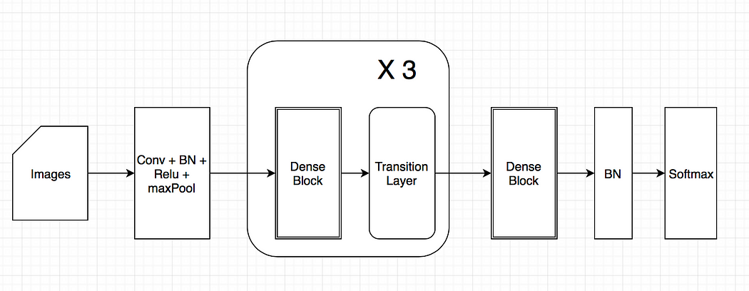
Figure 1 shows the DenseNet architecture.

Figure 1: DenseNet Architecture ⁶

As shown in Figure 1, DenseNet contains a feature layer (convolutional layer) capturing low-level features from images, several dense blocks, and transition layers between adjacent dense blocks ⁵.

3.1 Dense blocks

Dense block contains several dense layers. The depth of a dense layer output is called growth_rate. Every dense layer receives all the output of its previous layers. The input depth for the kth layer is (k-1)*growth_rate + input_depth_of_first_layer. By adding more layers in a dense block, the depth will grow linearly. For example, if the growth rate is 30 and after 100 layers, the depth will be over 3000. However, this could lead to a computational explosion. It is addressed by introducing a transition layer to reduce and abstract the features after a dense block with a limited number of dense layers to circumvent this problem ⁷. A 1x1 convolutional layer (bottleneck layer) is added to reduce the computation, which makes the second convolutional layer always has a fixed input depth. It is also easy to see the size (width and height) of the feature maps keeps the same through the dense layer, making it easy to stack any number of dense layers together to build a dense block. For example, densenet121 has four dense blocks with 6, 12, 24, and 16 dense layers. With repetition, it is not that difficult to make 112 layers ⁷.

3.2 Transition layers

In general, the size of every layer’s output in Convolutional Neural Network decreases to abstract higher-level features. In DenseNet, the transition layers take this responsibility while the dense blocks keep the size and depth. Every transition layer contains a 1x1 convolutional layer and a 2x2 average pooling layer to reduce the size to half. However, transition layers also receive all the output from all the last dense block layers. So the 1*1 convolutional layer reduces the depth to a fixed number, while the average pooling reduces the size.

4. Overview of CheXpert Dataset

CheXpert is a large public dataset. It contains an interpreted chest radiograph consisting of 224,316 chest radiographs of 65,240 patients labeled for the presence of 14 observations as positive, negative, or uncertain ⁸.

Figure 2 shows the CheXpert 14 labels and the Probability ⁹. Our analysis is to predict the probability of 5 different observations (Atelectasis, Cardiomegaly, Consolidation, Edema, and Pleural Effusion) from multi-view chest radiographs shown in Figure 2

Figure 2: Probability of different observations ⁹.

4.1 Data Collection

CheXpert dataset is a collection of chest radiographic studies from Stanford Hospital, performed between October 2002 and July 2017 in inpatient and outpatient centers, along with their associated radiology reports. Based on studies, a sampled set of 1000 reports were created for manual review by a board-certified radiologist to determine the feasibility for extraction of observations. The final set consists of 14 observations based on the prevalence in the reports and clinical relevance, conforming to the Fleischner Society’s recommended glossary. Pneumonia, despite being a clinical diagnosis, Pneumonia was included as a label to represent the images that suggested primary infection as the diagnosis. The No Finding observation was intended to capture the absence of all pathologies ⁸.

4.2 Data Labelling

Labels developed using an automated, rule-based labeler to extract observations from the free text radiology reports to be used as structured labels for the images ⁸.

4.3 Label Extraction

The labeler extracts the pathologies mentioned in the list of observations from the Impression section of radiology reports, summarizing the key findings in the radiographic study. Multiple board-certified radiologists manually curated a large list of phrases to match various observations mentioned in the reports ⁸.

4.4 Label Classification

Labeler extracts the mentions of observations and classify them as negative (“no evidence of pulmonary edema, pleural effusions or pneumothorax”), uncertain (“diffuse reticular pattern may represent mild interstitial pulmonary edema”), or positive (“moderate bilateral effusions and bibasilar opacities”). The ‘uncertain’ label can capture both the uncertainty of a radiologist in the diagnosis as well as the ambiguity inherent in the report (“heart size is stable”). The mention classification stage is a 3-phase pipeline consisting of pre-negation uncertainty, negation, and post-negation uncertainty. Each phase consists of rules that are matched against the mention; if a match is found, the mention is classified accordingly (as uncertain in the first or third phase and as negative in the second phase). If a mention is not matched in any of the phases, it is classified as positive ⁸.

4.5 Label Aggregation

CheXpert dataset use the classification for each mention of observations to arrive at a final label for 14 observations that consist of 12 pathologies and the “Support Devices” and “No Finding” observations. Observations with at least one mention positively classified in the report are assigned a positive (1) label. An observation is assigned an uncertain (u) label if it has no positively classified mentions and at least one uncertain mention, and a negative label if there is at least one negatively classified mention. We assign (blank) if there is no mention of an observation. The “No Finding” observation is assigned a positive label (1) if there is no pathology classified as positive or uncertain ⁸.

5. Overview Of AUC-ROC Curve

AUC-ROC stands for Area Under Curve - Receiver Operating Characteristics. It visualizes how well a machine learning classifier is performing. However, it works for only binary classification problems ¹⁰. In our project, we extend it to evaluate Multi-Image classification problem. AUC-ROC curve is a performance measurement for classification problems at various threshold settings. ROC is a probability curve, and AUC represents the degree or measure of separability. Higher the AUC, the better the model is at predicting 0s as 0s and 1s as 1s. By analogy, the Higher the AUC, the model distinguishes between patients with the disease and no disease ¹¹.

Figure 3 shows Confusion Matrix. We use Confusion Matrix to explain Sensitivity and Specificity.

Figure 3: Confusion Matrix

5.1 Sensitivity/True Positive Rate (TPR)

Sensitivity/True Positive Rate (TPR) explains what proportion of the positive class got correctly classified. A simple example would be determining what proportion of the actual sick people are correctly detected by the model ¹⁰.

5.2 False Negative Rate (FNR)

False Negative Rate (FNR) explains what proportion of the positive class is incorrectly classified by the classifier. A higher TPR and a lower FNR means correctly classify the positive class ¹⁰.

5.3 Specificity/True Negative Rate (TNR)

Specificity/True Negative Rate (TNR) indicates what proportion of the negative class is classified correctly. For example, Specificity determines what proportion of actual healthy people are correctly classified as healthy by the model ¹⁰.

5.4 False Positive Rate (FPR)

False Positive Rate (FPR) indicates what proportion of the negative class got incorrectly classified by the classifier. A higher TNR and a lower FPR means the model correctly classifies the negative class¹⁰.

5.5 Purpose of AUC-ROC curve

A machine learning classification model can predict the actual class of the data point directly or predict its probability of belonging to different classes. The example for the former case is where a model can classify whether a patient is healthy or not healthy. In the latter case, a model can predict a patient’s probability of being healthy or not healthy and provide more control over the result by enabling a way to tune the model’s behavior by changing the threshold values. This is powerful because it eliminates the possibility of building a completely new model to achieve a different range of results ¹⁰. A threshold value helps to interpret the probability and map the probability to a class label. For example, a threshold value such as 0.5, where all values equal to or greater than the threshold, is mapped to one class and rests to another class ¹².

Introducing different thresholds for classifying positive class for data points will inadvertently change the Sensitivity and Specificity of the model. Furthermore, one of these thresholds will probably give a better result than the others, depending on whether we aim to lower the number of False Negatives or False Positives ¹⁰. As seen in Figure 8, the metrics change with the changing threshold values. We can generate different confusion matrices and compare the various metrics. However, it is very inefficient. Instead, we can generate a plot between some of these metrics so that we can easily visualize which threshold is giving us a better result. The AUC-ROC curve solves just that ¹⁰.

Figure 8: Probability of prediction and metrics ¹⁰.

5.6 Definition of AUC-ROC

The Receiver Operator Characteristic (ROC) curve is an evaluation metric for binary classification problems. It is a probability curve that plots the TPR against FPR at various threshold values and essentially separates the signal from the noise. The Area Under the Curve (AUC) is the measure of a classifier’s ability to distinguish between classes and is used as a summary of the ROC curve. The higher the AUC, the better the model’s performance at distinguishing between the positive and negative classes. When AUC = 1, the classifier can perfectly distinguish between all the Positive and the Negative class points correctly. If, however, the AUC had been 0, then the classifier would be predicting all Negatives as Positives and all Positives as Negatives. When 0.5<AUC<1, there is a high chance that the classifier will be able to distinguish the positive class values from the negative class values. This is because the classifier can detect more True positives and True negatives than False negatives and False positives. When AUC=0.5, then the classifier is not able to distinguish between Positive and Negative class points. It means either the classifier is predicting random class or constant class for all the data points. Therefore, the higher the AUC value for a classifier, the better its ability to distinguish between positive and negative classes. In the AUC-ROC curve, a higher X-axis value indicates a higher number of False positives than True negatives. Simultaneously, a higher Y-axis value indicates a higher number of True positives than False negatives. So, the choice of the threshold depends on balancing between False positives and False negatives ¹⁰.

6. Chest X-Rays - Multi-Image Classification Using Deep Learning Model

Our Deep Learning model loads and processes the raw data files and implement a Python class to represent data by converting it into a format usable by PyTorch. We then, visualize the training and validation data.

Our approach to predicting pathologies will have 5 steps.

• Load and split Chest X-rays Dataset
• Build and train baseline Deep Learning model
• Evaluate the model
• Predict the pathologies
• Calculate the AUC-ROC score

6.1 Load and split Chest X-rays Dataset

We load and split the dataset to 90% for training and 10% for validation randomly.

6.2 Build and train baseline Deep Learning model

We use the PyTorch library to implement and train DenseNet CNN as a baseline model. With initial weights from ImageNet, we retrain all layers. In PyTorch, we implement a subclass for the PyTorch to transform CheXpert Dataset and create a custom data loading process. The Image Augmentation is executed within this subclass. Additionally, a DataLoader also needs to be created. We shuffle the dataset for the training dataloader. We also create a validation dataloader, which is different from the training dataloader and does not require shuffling. In the baseline model, we use DenseNet pre-trained on the ImageNet dataset. The model’s classifier is replaced with a new dense layer and use the CheXpert labels to train ¹¹. The number of trainable parameters 6968206 (~7 million).

6.3 Evaluate the model

To evaluate the model, we implement a function to validate the model on the validation dataset.

6.4 Predict the pathologies

We use our model to predict 1 of the 5 pathologies - Atelectasis, Cardiomegaly, Consolidation, Edema, and Pleural Effusion. Our model uses a test dataset.

6.5 Calculate the AUC-ROC score

We have multiple labels, and we need to calculate the AUCROC-score for each class against the rest of the classifiers.

7. Results and Analysis

Figure 9 shows training loss, Validation loss and validation AUC-ROC score after training our Deep Learning model for 7 hours.

Figure 9: Training loss, Validation loss and validation AUC-ROC score

Figure 10 shows model predicts False Positives. Below is AUCROC table.

Figure 10: AUC - ROC data

This graph is taken from Stanford CheXpert dataset. Based on Figure 11 ¹³, our AUCROC value is around 85%.

Figure 11: AUC - ROC Curve ¹³

8. Conclusion

Our model achieves the best AUC on Edema (0.89) and the worst on Plural(0.65). The AUC of all other observations is around 0.78. Our model achieves above 0.65 overall predictions.

9. Future Plans

As the next steps, we will work to improve the model’s algorithm and leverage DenseNet architecture to train using smaller dataset.

10. Acknowledgements

The author would like to thank Dr. Gregor Von Laszewski, Dr. Geoffrey Fox, and the associate instructors for providing continuous guidance and feedback for this final project.

11. References

12. Appendix

12.1 Project Plan

• October 26, 2020
  • Test train and validate functionality on PyTorch Dataset
  • Update Project.md with project plan
• November 02, 2020
  • Test train and validate functionality on manual uploaded CheXpert Dataset
  • Update project.md with specific details about Deep learning models
• November 09, 2020
  • Test train and validate functionality on downloaded CheXpert Dataset using “wget”
  • Update project.md with details about train and validation data set
  • Capture improvements to loss function
• November 16, 2020
  • Self review - code and project.md
• December 02, 2020
  • Review with TA/Professor - code and project.md
• December 07, 2020
  • Final submission - code and project.md