Python is a great languge for doing data science and AI, a comprehensive list of features is available in book form. Please note that when installing Python, you always want to use a venv as this is best practice.

Introduction to Python (ePub) (PDF)

Installation of Python

Installation of Python — June 7th, 2021 (AM)

Update to the Video:

Best practices in Python recommend to use a Python venv. This is pretty easy to do and creates a separate Python environment for you so you do not interfere with your system Python installation. Some IDEs may do this automatically, but it is still best practice to install one and bind the IDE against it. To do this:

Download Python version 3.9.5 just as shown in the first lecture.
After the download you do an additional step as follows:
- on Mac:
```
python3.9 -m venv ~/ENV3
source ~/ENV/bin/activate
```
  you need to do the source every time you start a new window or on mac ass it to .zprofile

on Windows you first install gitbash and do all yuour terminal work from gitbash as this is more Linux-like. In gitbash, run
```
python -m venv ~/ENV3
~/ENV/Script/activate
```
In case you like to add it to gitbash, you can add the source line to .bashrc and/or .bash_profile

In case you use VSCode, you can also do it individually in a directory where you have your code.
- On Mac: cd TO YOUR DIR; python3.9 -m venv .
- On Windows cd TO YOUR DIR; python -m venv .
Then start VSCode in the directory and it will ask you to use this venv. However, the global ENV3 venv may be better and you cen set your interpreter to it.
On Pycharm we recommend you use the ENV3 and set the clobal interpreter

Jupyter Notebooks

Jupyter Notebooks — June 7th, 2021 (PM): This lecture provides an introduction to Jupyter Notebooks using Visual Studio as IDE.

Github

Video: Github

Video-Github 2 — June 8th, 2021 (PM): In this lecture the student can learn how to create a project on RStudio and link it with a repository on GitHub to commit, pull and push the code from RStudio.

Introduction to Python

Slides: This introduction to Python cover the different data type, how to convert type of variable, understand and create flow control usign conditional statements.

Video-Introduction to Python (1) — June 9th, 2021 (AM): This introduction to Python cover the different data type, how to convert type of variable, understand and create flow control usign conditional statements.

Video-Introduction to Python (2) — June 9th, 2021 (PM): This introduction to Python cover the different data type, how to convert type of variable, understand and create flow control usign conditional statements.

Video-Introduction to Python (3) — June 10th, 2021 (AM): This lecture introduces the use of Google Colab to code your python program using the resources provided by Google. Also, DataFrame is introduced and use to manipulate and analyze data.

Slides — June 10th, 2021 (PM): String, Numbers, Booleans Flow of control Using If statements

Slides: String, Numbers, Booleans Flow of control Using If statements (2)

Python Exercises - Lab 2

The first exercise will require a simple for loop, while the second is more complicated, requiring nested for loops and a break statement.

General Instructions: Create two different files with extension .ipnyb, one for each problem. The first file will be named factorial.ipnyb which is for the factorial problem, and the second prime_number.ipnyb for the prime number problem.

Write a program that can find the factorial of any given number. For example, find the factorial of the number 5 (often written as 5!) which is 12345 and equals 120. Your program should take as input an integer from the user.

Note: The factorial is not defined for negative numbers and the factorial of Zero is 1; that is 0! = 1.

You should
1. If the number is less than Zero return with an error message.
2. Check to see if the number is Zero—if it is then the answer is 1—print this out.
3. Otherwise use a loop to generate the result and print it out.
A Prime Number is a positive whole number, greater than 1, that has no other divisors except the number 1 and the number itself. That is, it can only be divided by itself and the number 1, for example the numbers 2, 3, 5 and 7 are prime numbers as they cannot be divided by any other whole number. However, the numbers 4 and 6 are not because they can both be divided by the number 2 in addition the number 6 can also be divided by the number 3.

You should write a program to calculate prime number starting from 1 up to the value input by the user.

You should
1. If the user inputs a number below 2, print an error message.
2. For any number greater than 2 loop for each integer from 2 to that number and determine if it can be divided by another number (you will probably need two for loops for this; one nested inside the other).
3. For each number that cannot be divided by any other number (that is its a prime number) print it out.

Motivation for the REU

Video — June 11th, 2021 (AM): Motivation for the REU: Data is Driven Everything

Slides: Motivation for the REU: Data is Driven Everything

Slides: Descriptive Statistic

Slides: Probability

Video — June 28th, 2021 (AM): Working on GitHUb Template and Mendeley references management

Data Science Tools

Slides: Data Science Tools

Video — June 14th, 2021 (AM): Numpy

Video — June 14th, 2021 (PM): Pandas data frame

Video — June 15th, 2021 (AM): Web data mining

Video — June 15th, 2021 (PM): Pandas IO

Video — June 16th, 2021 (AM): Pandas

Video-Matrix computation — June 16th, 2021 (PM): Linear algebra is a main compornent in the field of Data Science. As a consequence, this lecture introduces the main matrix operations such as, addition, substraction, multiplication, and picewise multiplication.

Video: Pycharm Installation and Virtual Environment setup — June 18th, 2021 (AM)

Application of Matrix Operation using Images on Python

Video: This lecture the student can learn the different applications of Matrix Operation using images on Python. — June 21st, 2021 (AM)

Video: Data wrangling and Descriptive Statistic Using Python — June 21st, 2021 (AM)

Video: Data wrangling and Descriptive Statistic Using Python — June 22nd, 2021 (PM)

Video: FURY Visualization and Microsoft Lecture — June 25th, 2021 (PM)

Video: Instroduction to Probability — June 25th, 2021 (PM)

Video: Digital Twins and Virtual Tissue ussing CompuCell3D Simulating Cancer Somatic Evolution in nanoHUB — July 2nd, 2021 (AM)

AI First Engineering

Video: AI First Engineering: Learning material — June 25th, 2021 (AM)

Adding content to your su21-reu repositorirs

Video: Adding content to your su21-reu repositories — June 17th, 2021 (PM)

Slides: AI First Engineering

Datasets for Projects

Video: Datasets for Projects: Data world and Kaggle — June 29th, 2021 (AM)

Video: Datasets for Projects: Data world and Kaggle part 2 — June 29th, 2021 (PM)

Machine Learning Models

Video: K-Means: Unsupervised model — June 30th, 2021 (AM)

Video: Support Vector Machine: Supervised model — July 2nd, 2021 (PM)

Slides: Support Vector Machine Supervised model.

Video: Neural Networks: Deep Learning Supervised model — July 6th, 2021 (AM)

SVideo: Neural Networks: Deep learning Model

Video: Neural Networks: Deep learning Model — July 6th, 2021 (AM)

Video: Data Visualization: Visualizaton for Data Science — July 7th, 2021 (AM)

Video: Convulotional Neural Networks: Deep learning Model — July 8th, 2021 (AM)

Students Report Help

Video: Student Report Help with Introduction and Datasets — July 7th, 2021 (AM)

Video: Student Report Help with Introduction and Datasets — July 13th, 2021 (AM)

COVID-19

Video: Chemo-Preventive Effect of Vegetables and Fruits Consumption on the COVID-19 Pandemic — July 1st, 2021 (AM)

1.2 - AI-First Engineering Cybertraining

This course introduces the students to AI-First principles. The notes are prepared for the course taught in 2021.

This is an image

This course introduces the students to AI-First Engineering Cybertraining we provide the following sections

Class Material

As part of this class, we will be using a variety of sources. To simplify the presentation we provide them in a variety of smaller packaged material including books, lecture notes, slides, presentations and code.

Note: We will regularly update the course material, so please always download the newest version. Some browsers try to be fancy and cache previous page visits. So please make sure to refresh the page.

We will use the following material:

Course Lectures and Management

Course Lectures. These meeting notes are updated weekly (Web)

Overview

This course is built around the revolution driven by AI and in particular deep learning that is transforming all activities: industry, research, and lifestyle. It will a similar structure to The Big Data Class and the details of the course will be adapted to the interests of participating students. It can include significant deep learning programming.

All activities – Industry, Research, and Lifestyle – are being transformed by Artificial Intelligence AI and Big Data. AI is currently dominated by deep learning implemented on a global pervasive computing environment - the global AI supercomputer. This course studies the technologies and applications of this transformation.

We review Core Technologies driving these transformations: Digital transformation moving to AI Transformation, Big Data, Cloud Computing, software and data engineering, Edge Computing and Internet of Things, The Network and Telecommunications, Apache Big Data Stack, Logistics and company infrastructure, Augmented and Virtual reality, Deep Learning.

There are new “Industries” over the last 25 years: The Internet, Remote collaboration and Social Media, Search, Cybersecurity, Smart homes and cities, Robotics. However, our focus is Traditional “Industries” Transformed: Computing, Transportation: ride-hailing, drones, electric self-driving autos/trucks, road management, travel, construction Industry, Space, Retail stores and e-commerce, Manufacturing: smart machines, digital twins, Agriculture and Food, Hospitality and Living spaces: buying homes, hotels, “room hailing”, Banking and Financial Technology: Insurance, mortgage, payments, stock market, bitcoin, Health: from DL for pathology to personalized genomics to remote surgery, Surveillance and Monitoring: – Civilian Disaster response; Miltary Command and Control, Energy: Solar wind oil, Science; more data better analyzed; DL as the new applied mathematics, Sports: including Sabermetrics, Entertainment, Gaming including eSports, News, advertising, information creation and dissemination, education, fake news and Politics, Jobs.

We select material from above to match student interests.

Students can take the course in either software-based or report-based mode. The lectures with be offered in video form with a weekly discussion class. Python and Tensorflow will be main software used.

Lectures on Particular Topics

Introduction to AI-Driven Digital Transformation

Introduction to AI-Driven Digital Transformation (Web)

Introduction to Google Colab

A Gentle Introduction to Google Colab (Web)

A Gentle Introduction to Python on Google Colab (Web)

MNIST Classification on Google Colab (Web)

MNIST Classification with MLP on Google Colab (Web)

MNIST-MLP Classification on Google Colab (Web)

MNIST Classification with RNN on Google Colab (Web)

MNIST-RNN Classification on Google Colab (Web)

MNIST Classification with LSTM on Google Colab (Web)

MNIST-LSTM Classification on Google Colab (Web)

MNIST Classification with Autoencoder on Google Colab (Web)

MNIST-Autoencoder Classification on Google Colab (Web)

MNIST with MLP+LSTM Classification on Google Colab (Web)

Distributed Training with MNIST Classification on Google Colab (Web)

PyTorch with MNIST Classification on Google Colab (Web)

Material

Complementary Material

When working with books, ePubs typically display better than PDF. For ePub, we recommend using iBooks on macOS and calibre on all other systems.

Piazza

Piazza. The link for all those that participate in the IU class to its class Piazza.

Scientific Writing with Markdown

Scientific Writing with Markdown (ePub) (PDF)

Git Pull Request

Git Pull Request. Here you will learn how to do a simple git pull request either via the GitHub GUI or the git command line tools

Introduction to Linux

This course does not require you to do much Linux. However, if you do need it, we recommend the following as starting point listed

The most elementary Linux features can be learned in 12 hours. This includes bash, editor, directory structure, managing files. Under Windows, we recommend using gitbash, a terminal with all the commands built-in that you would need for elementary work.

Introduction to Linux (ePub) (PDF)

Older Course Material

Older versions of the material are available at

Lecture Notes 2020 (ePub) (PDF)

Big Data Applications (Nov. 2019) (ePub) (PDF)

Big Data Applications (2018) (ePub) (PDF)

Contributions

You can contribute to the material with useful links and sections that you find. Just make sure that you do not plagiarize when making contributions. Please review our guide on plagiarism.

Computer Needs

This course does not require a sophisticated computer. Most of the things can be done remotely. Even a Raspberry Pi with 4 or 8GB could be used as a terminal to log into remote computers. This will cost you between $50 - $100 dependent on which version and equipment. However, we will not teach you how to use or set up a Pi or another computer in this class. This is for you to do and find out.

In case you need to buy a new computer for school, make sure the computer is upgradable to 16GB of main memory. We do no longer recommend using HDD’s but use SSDs. Buy the fast ones, as not every SSD is the same. Samsung is offering some under the EVO Pro branding. Get as much memory as you can effort. Also, make sure you back up your work regularly. Either in online storage such as Google, or an external drive.

1.2.1 - Project Guidelines

We present here the AI First Engineering project guidelines

We present here the project guidelines

All students of this class are doing a software project. (Some of our classes allow non software projects)

The final project is 50% of grade
All projects must have a well-written report as well as the software component
We must be able to run software from class GitHub repository. To do so you must include an appendix to your project report describing how to run your project.
- If you use containers you must decsribe how to create them from Docker files.
- If you usue ipy notebooks you must include a button or links so it can be run in Google collab
There are a useful set of example projects submitted in previous classes
- Last year’s Fall 2020 Big Data class
- Earlier Classes [https://github.com/cybertraining-dsc/pub/blob/master/docs/vonLaszewski-cloud-vol-9.pdf] (26 projects)
- Earlier Classes [https://github.com/cybertraining-dsc/pub/blob/master/docs//vonLaszewski-i523-v3.pdf] (45 projects)
- Earlier Classes [https://github.com/cybertraining-dsc/pub/blob/master/docs//vonLaszewski-i524-spring-2017.pdf] (28 projects)
In this class you do not have the option to work on a joint report, however you can collaborate.
Note: all reports and projects are open for everyone as they are open source.

Details

The major deliverable of the course is a software project with a report. The project must include a programming part to get a full grade. It is expected that you identify a suitable analysis task and data set for the project and that you learn how to apply this analysis as well as to motivate it. It is part of the learning outcome that you determine this instead of us giving you a topic. This topic will be presented by student in class April 1.

It is desired that the project has a novel feature in it. A project that you simply reproduce may not recieve the best grade, but this depends on what the analysis is and how you report it.

However “major advances” and solving of a full-size problem are not required. You can simplify both network and dataset to be able to complete project. The project write-up should describe the “full-size” realistic problem with software exemplifying an instructive example.

One goal of the class is to use open source technology wherever possible. As a beneficial side product of this, we are able to distribute all previous reports that use such technologies. This means you can cite your own work, for example, in your resume. For big data, we have more than 1000 data sets we point to.

Comments on Example Projects from previous classes

Warning: Please note that we do not make any quality assumptions to the published papers that we list here. It is up to you to identify outstanding papers.

Warning: Also note that these activities took place in previous classes, and the content of this class has since been updated or the focus has shifted. Especially chapters on Google Colab, AI, DL have been added to the course after the date of most projects. Also, some of the documents include an additional assignment called Technology review. These are not the same as the Project report or review we refer to here. These are just assignments done in 2-3 weeks. So please do not use them to identify a comparison with your own work. The activities we ask from you are substantially more involved than the technology reviews.

Format of Project

Plagiarism is of course not permitted. It is your responsibility to know what plagiarism is. We provide a detailed description book about it here, you can also do the IU plagiarism test to learn more.

All project reports must be provided in github.com as a markdown file. All images must be in an images directory. You must use proper citations. Images copied from the Internet must have a citation in the Image caption. Please use the IEEE citation format and do not use APA or harvard style. Simply use fotnotes in markdown but treat them as regular citations and not text footnotes (e.g. adhere to the IEEE rules).
All projects and reports must be checked into the Github repository. Please take a look at the example we created for you.

The report will be stored in the github.com.

./project/index.md

./project/images/mysampleimage.png

Length of Project Report

Software Project Reports: 2500 - 3000 Words.

Possible sources of datasets

Given next are links to collections of datasets that may be of use for homework assignments or projects.

FAQ

Why you should not just paste and copy into the GitHub GUI?

We may make comments directly in your markdown or program files. If you just paste and copy you may overlook such comments. HEns only paste and copy small paragraphs. If you need to. The best way of using github is from commandline and using editors such as pycharm and emacs.
I like to do a project that relates to my company?
- Please go ahead and do so but make sure you use open-source data, and all results can be shared with everyone. If that is not the case, please pick a different project.
Can I use Word or Google doc, or LaTeX to hand in the final document?
- No. you must use github.com and markdown.
- Please note that exporting documents from word or google docs can result in a markdown file that needs substantial cleanup.
Where do I find more information about markdown and plagiarism
https://laszewski.github.io/publication/las-20-book-markdown/
[https://cloudmesh-community.github.io/pub/vonLaszewski-writing.pdf]{.ul}
Can I use an online markdown editor?
- There are many online markdown editors available. One of them is [https://dillinger.io/]{.ul}.
  Use them to write your document or check the one you have developed in another editor such as word or google docs.
- Remember, online editors can be dangerous in case you lose network connection. So we recommend to develop small portions and copy them into a locally managed document that you then check into github.com.
- Github GUI (recommended): this works very well, but the markdown is slightly limited. We use hugo’s markdown.
- pyCharm (recommended): works very well.
- emacs (recommended): works very well
What level of expertise and effort do I need to write markdown?
- We taught 10-year-old students to use markdown in less than 5 minutes.
What level of expertise is needed to learn BibTeX
- We have taught BibTeX to inexperienced students while using jabref in less than an hour (but it is not required for this course). You can use footnotes while making sure that the footnotes follow the IEEE format.
How can I get IEEE formatted footnotes?
- Simply use jabref and paste and copy the text it produces.
Will there be more FAQ’s?
- Please see our book on markdown.
- Discuss your issue in piazza; if it is an issue that is not yet covered, we will add it to the book.
How do I write URLs?
- Answered in book
- Note: All URL’s must be either in [TEXT](URLHERE) or <URLHERE> format.

1.3 - Big Data 2020

This course introduces the students to Cloud Big Data Applications. The notes are prepared for the course taught in 2020.

This is an image

This course introduces the students to Cloud Big Data Applications we provide the following sections

Class Material

We will use the following material:

Course Lectures and Management

Course Lectures. These meeting notes are updated weekly (Web)

Lectures on Particular Topics

Introduction to AI-Driven Digital Transformation

Introduction to AI-Driven Digital Transformation (Web)

Big Data Usecases Survey

This module covers 51 usecases of Big data that emerged from a NIST (National Institute for Standards and Technology) study of Big data. We cover the NIST Big Data Public Working Group (NBD-PWG) Process and summarizes the work of five subgroups: Definitions and Taxonomies Subgroup, Reference Architecture Subgroup, Security and Privacy Subgroup, Technology Roadmap Subgroup and the Requirements andUse Case Subgroup. 51 use cases collected in this process are briefly discussed with a classification of the source of parallelism and the high and low level computational structure. We describe the key features of this classification.

Introduction to Google Colab

A Gentle Introduction to Google Colab (Web)

A Gentle Introduction to Python on Google Colab (Web)

MNIST Classification on Google Colab (Web)

Material

Physics

Big Data Applications and Analytics Discovery of Higgs Boson Part I (Unit 8) Section Units 9-11 Summary: This section starts by describing the LHC accelerator at CERN and evidence found by the experiments suggesting existence of a Higgs Boson. The huge number of authors on a paper, remarks on histograms and Feynman diagrams is followed by an accelerator picture gallery. The next unit is devoted to Python experiments looking at histograms of Higgs Boson production with various forms of shape of signal and various background and with various event totals. Then random variables and some simple principles of statistics are introduced with explanation as to why they are relevant to Physics counting experiments. The unit introduces Gaussian (normal) distributions and explains why they seen so often in natural phenomena. Several Python illustrations are given. Random Numbers with their Generators and Seeds lead to a discussion of Binomial and Poisson Distribution. Monte-Carlo and accept-reject methods. The Central Limit Theorem concludes discussion.

Sports

Sports sees significant growth in analytics with pervasive statistics shifting to more sophisticated measures. We start with baseball as game is built around segments dominated by individuals where detailed (video/image) achievement measures including PITCHf/x and FIELDf/x are moving field into big data arena. There are interesting relationships between the economics of sports and big data analytics. We look at Wearables and consumer sports/recreation. The importance of spatial visualization is discussed. We look at other Sports: Soccer, Olympics, NFL Football, Basketball, Tennis and Horse Racing.

Health and Medicine

AI in Banking

Transportation Systems

Transportation systems is a vital component in human life. With the dawn of AI, transportation systems are also reinforced to provide better service for the people. Analyzing tera-bytes of data collected in day-to-day transportation activities are used to analyze issues and provide a better experience for the user.

Space and Energy

Mobility (Industry)

Cloud Computing

Commerce

Complementary Material

When working with books, ePubs typically display better than PDF. For ePub, we recommend using iBooks on macOS and calibre on all other systems.

Piazza

Piazza. The link for all those that participate in the IU class to its class Piazza.

Scientific Writing with Markdown

Scientific Writing with Markdown (ePub) (PDF)

Git Pull Request

Git Pull Request. Here you will learn how to do a simple git pull request either via the GitHub GUI or the git command line tools

Introduction to Linux

This course does not require you to do much Linux. However, if you do need it, we recommend the following as starting point listed

Introduction to Linux (ePub) (PDF)

Older Course Material

Older versions of the material are available at

Lecture Notes 2020 (ePub) (PDF)

Big Data Applications (Nov. 2019) (ePub) (PDF)

Big Data Applications (2018) (ePub) (PDF)

Contributions

You can contribute to the material with useful links and sections that you find. Just make sure that you do not plagiarize when making contributions. Please review our guide on plagiarism.

Computer Needs

1.4 - REU 2020

This course introduces the REU students to various topics in Intelligent Systems Engineering. The course was taught in Summer 2020.

Computational Foundations

Brief Overview of the Praxis AI Platform and Overview of the Learning Paths
Accessing Praxis Cloud
Introduction To Linux and the Command Line
Jupyter Notebooks
A Brief Intro to Machine Learning in Google Colaboratory

Programming with Python

Selected chapters from out python Book

Analyzing Patient Data
Loops Lists Analyzing Data
Functions Errors Exceptions
Defensive Programming Debugging

Introduction to Python (ePub) (PDF)

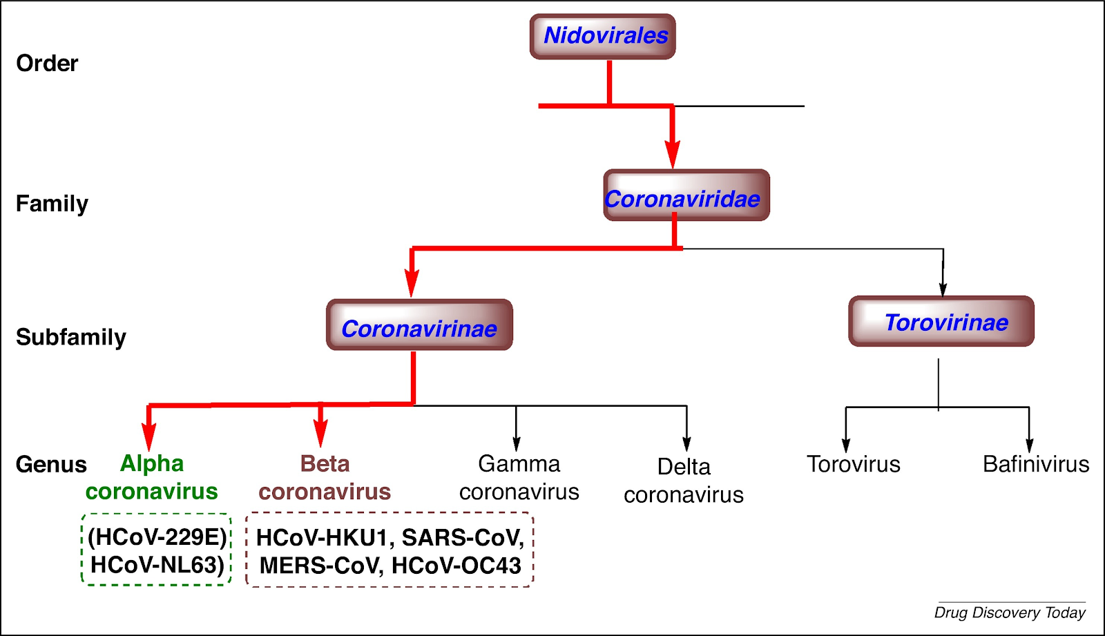
Coronavirus Overview

Basic Virology and Immunology

Case Study: 1918 Influenza Pandemic: Prior to COVID-19, the 1918 influenza pandemic was the most severe pandemic in recent history. First identified in military personnel in the spring of 1918, the influenza was an H1N1 virus of avian origin. It is commonly referred to by scientists and historians as “the Mother of all Pandemics.” This pandemic is often referred to as the “Spanish Flu” in the lay press, though this name is a misnomer, and the virus likely originated elsewhere. Contemporary reporting focused heavily on Spain, as it was one of few places at the time that did not have restrictions on the press during World War I.

SnapShot: COVID-19: In December 2019, several cases of pneumonia of unknown origin were reported in Wuhan, China. The causative agent was characterized as a novel coronavirus, initially referred to as 2019-nCoV and renamed severe acute respiratory syndrome coronavirus-2 (SARS-CoV-2) (Zhou et al., 2020b). This respiratory illness, coronavirus disease 2019 (COVID-19), has spread rapidly by human-to-human transmission, caused major outbreaks worldwide, and resulted in considerable morbidity and mortality. On March 11, 2020, WHO classified COVID-19 as a pandemic. It has stressed health systems and the global economy, as governments balance prevention, clinical care, and socioeconomic challenges.

Basic Virology and Immunology: In December 2019, a series of cases of pneumonia of unknown origin were reported in Wuhan, the capital city of Hubei province in China. The causative virus was isolated and characterized in January 2020 (Zhou et al., Nature 2020, Zhu et al., NEJM 2020). On January 12, 2020, the World Health Organization (WHO) tentatively named the virus as the 2019 novel coronavirus (2019-nCoV). On January 30, 2020 WHO issued a public health emergency of international concern (PHEIC) and on February 11, 2020, the WHO formally named the disease caused by the novel coronavirus as coronavirus disease 2019 (COVID-19). At that time, based on its genetic relatedness to known coronaviruses and established classification system, the International Committee on Taxonomy of Viruses classified and renamed 2019-nCoV as severe acute respiratory syndrome coronavirus 2 (SARS-CoV-2). On March 11, 2020, the WHO formally characterized the global spread of COVID-19 as a pandemic, the first to be caused by a coronavirus.

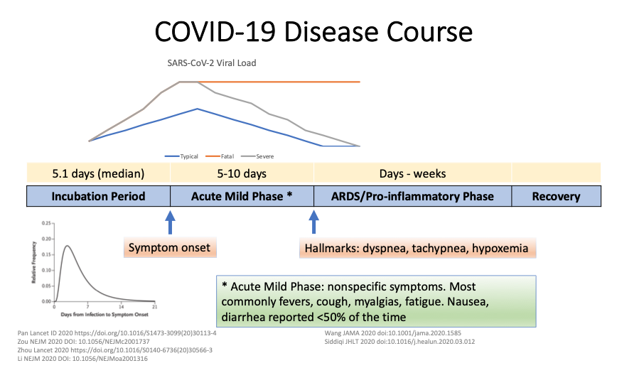
Clinical Presentation

Management of COVID-19

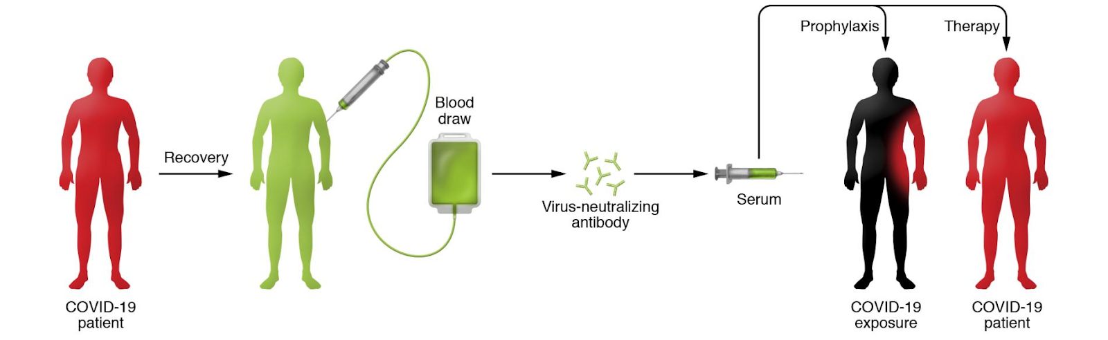
Investigational Therapeutics and Vaccine Development

Coronavirus Genomics Superlab

Pull from Computational Biology Journey

SARS by the numbers

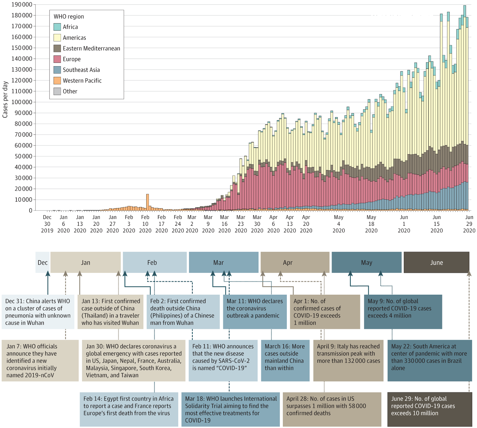
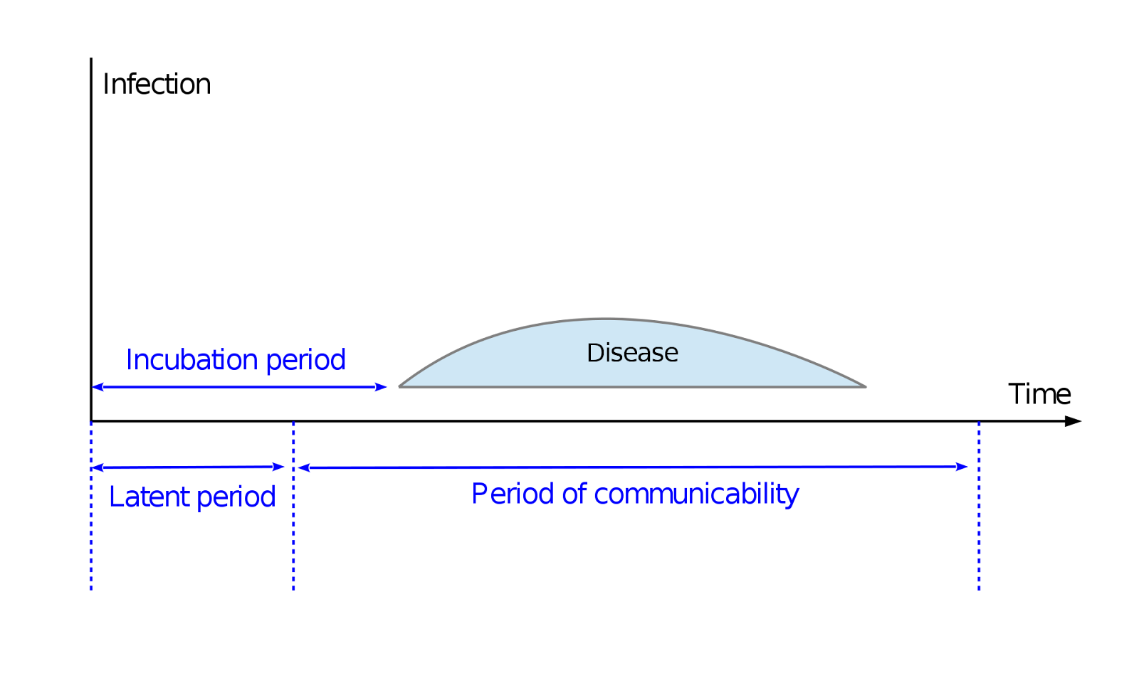
Epidemiology

Introduction to Epidemiological Terms

Principals

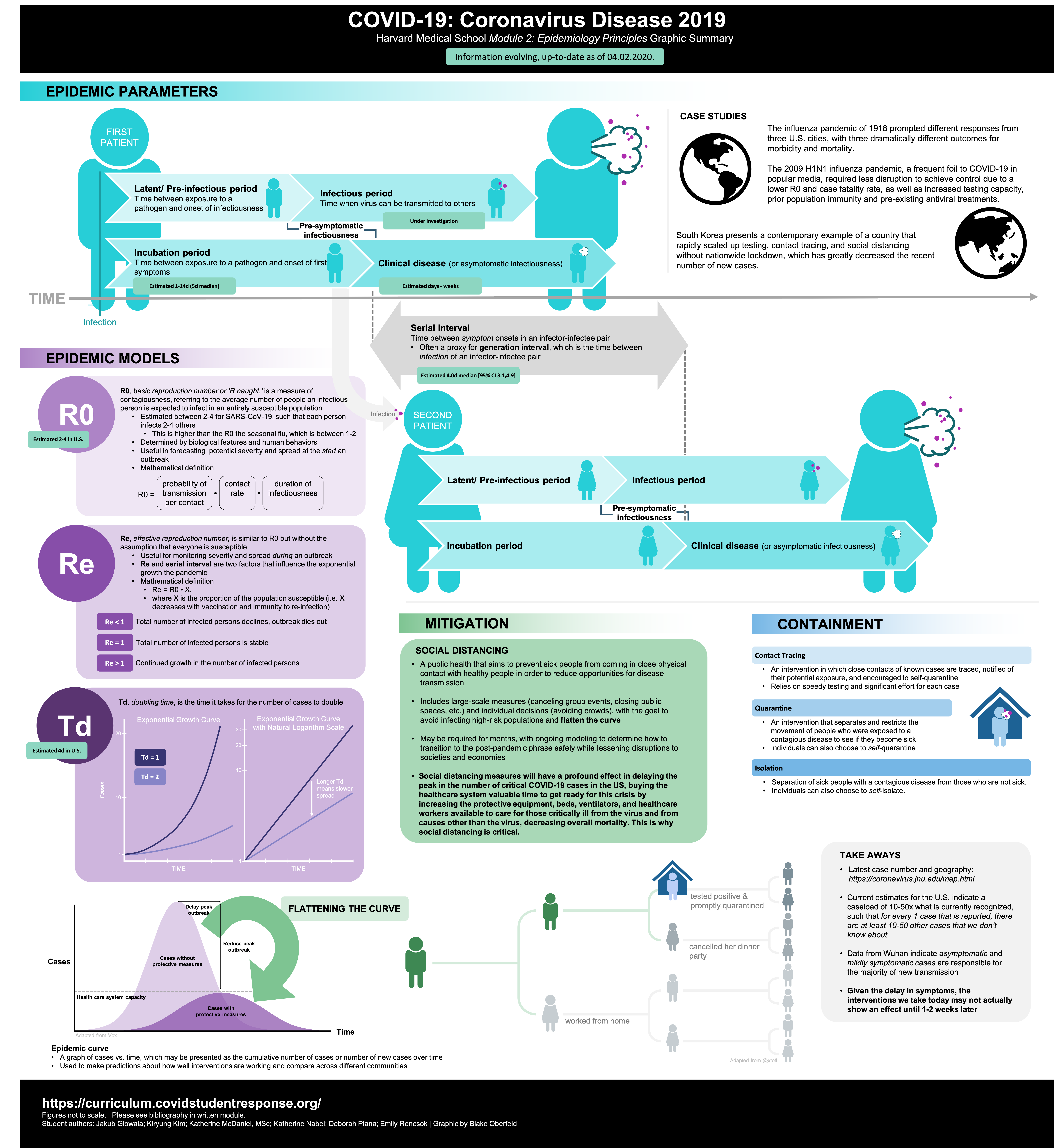
Summary

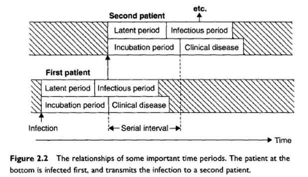
Introduction

Where Are We Now?

Where Will We Be Next?

Approaches to Long-Term Planning

Case Studies

1918-influenza-pandemic

2009 H1N1 pandemic

Soutch Korea 2020

Introduction to AI/Deep Learning

Deep Learning in Health and Medicine A: Overall Trends

Deep Learning in Health and Medicine B: Diagnostics

Deep Learning in Health and Medicine C: Examples

Deep Learning in Health and Medicine D: Impact of Corona Virus Covid-19

Deep Learning in Health and Medicine E: Corona Virus Covid-19 and Recession

Deep Learning in Health and Medicine F: Tackling Corona Virus Covid-19

Deep Learning in Health and Medicine G: Data and Computational Science and The Corona Virus Covid-19

Deep Learning in Health and Medicine H: Screening Covid-19 Drug Candidates

Deep Learning in Health and Medicine I: Areas for Covid19 Study and Pandemics as Complex Systems

REU Projects

REU Individual Project Overview and Expectations
Accessing the Coronavirus Datasets
Primer on How to Analyze the Data

Effect of AI on Industry and its Transformation Introduction to AI First Engineering

Examples of Applications of Deep Learning

Optimization – a key goal of Statistics, AI and Deep Learning

Learn the Deep Learning important words/components

Deep Learning and Imaging: It’s first greast success

For the BIg Data Class we revised the following material Big Data Overview Fall 2019

Big Data, technology, clouds and selected applications

20 Videos covering Big Data, technology, clouds and selected applications

Cloud Computing

18 Videos covering cloud computing

1.5 - Big Data 2019

This coursebook introduces the students to Cloud Big Data Applications

The document is available as an online book in ePub and PDF

For ePub, we recommend using iBooks on macOS and calibre on all other systems.

1.6 - Cloud Computing

This is a large volume that introduces you to many aspects of cloud computing.

The document is available as an online book in ePub and PDF from the following Web Page:

https://laszewski.github.io/book/cloud/

For ePub, we recommend using iBooks on Macos and calibre on all other systems.

THe book has over 590 pages. Topics coverd include:

DEFINITION OF CLOUD COMPUTING
CLOUD DATACENTER
CLOUD ARCHITECTURE
CLOUD REST
- NIST
- GRAPHQL
HYPERVISOR
- Virtualization
  - Virtual Machine Management with QEMU
IAAS
- Multipass
- Vagrant
- Amazon Web Services
- Microsoft Azure
- Google IaaS Cloud Services
- OpenStack
- Python Libcloud
- AWS Boto
- Cloudmesh
MAPREDUCE
- HADOOP
- SPARK
- HADOOP ECOSYSTEM
- TWISTER
- HADOOP RDMA
CONTAINERS
- DOCKER
- KUBERNETES
- Singularity
SERVERLESS
- FaaS
- Apache OpenWhisk
- Kubeless
- OpenFaaS ` * OpenLamda
MESSAGING
- MQTT
- Apache Avro
GO

1.7 - Data Science to Help Society

In this module, we will learn how to apply data science for the good of society. We introduce two examples, one for COVID-19, the other for hydrology.

COVID 101, Climate Change and their Technologies

General Material

Python Language

Need to add material here

Using Google CoLab and Jupyter notebooks

For questions on software, please mail Fugang Wang
- Fugang can also give you help on python including introductory material if you need extra
5 notebooks from Google
Introduction to Machine Learning Using TensorFlow (pptx)
Introduction to using Colab from IU class E534 with videos and note (google docs) This unit includes 3 videos
- How to create a colab notebook (mp4)
- How to create a simple program (mp4)
- How to do benchmark (mp4)
Deep Learning for MNIST The docs are located alongside the video at
- Introduction to MNIST
- This teaches how to do deep learning on a handwriting example from NIST which is used in many textbooks
- In the latter part of the document, a homework description is given. That can be ignored!
- There are 5 videos
  1. DNN MNIST Introduction (mp4)
  2. DNN MNIST import section (mp4)
    - Running into import errors starting at the keras.models line in the code
  3. DNN MNIST data preprocessing (mp4)
  4. DNN MNIST model definition (mp4)
  5. DNN MNIST final presentation (mp4)
Jupyter notebook on Google Colab for COVID-19 data analysis ipynb

Follow-up on Discussion of AI remaking Industry worldwide

Class on AI First Engineering with 35 videos describing technologies and particular industries Commerce, Mobility, Banking, Health, Space, Energy in detail (youtube playlist)
Introductory Video (one of 35) discussing the Transformation - Industries invented and remade through AI (youtube)
Some online videos on deep learning
- Introduction to AI First Engineering (youtube)

Examples of Applications of Deep Learning (youtube)

Optimization -- a key in Statistics, AI and Deep Learning (youtube)

Learn the Deep Learning important words and parts (youtube)

Deep Learning and Imaging: It's first great success (youtube)

Covid Material

Covid Biology Starting point

Medical Student COVID-19 Curriculum - COVID-19 Curriculum Module 1 and then module 2

Compucell3D Modelling material

Download
Manual
List of NanoHub Tools
For help please ask Juliano Ferrari Gianlupi

Interactive Two-Part Virtual Miniworkshop on Open-Source CompuCell3D

Multiscale, Virtual-Tissue Spatio-Temporal Simulations of COVID-19 Infection, Viral Spread and Immune Response and Treatment Regimes** VTcovid19Symp

Part I: Will be presented twice:
First Presentation June 11th, 2020, 2PM-5PM EST (6 PM- 9PM GMT)
Second Presentation June 12th, 9AM - 12 noon EST (1 PM - 4 PM GMT)
Part II: Will be presented twice:
First Presentation June 18th, 2020, 2PM-5PM EST (6 PM- 9PM GMT)
Second Presentation June 19th, 9AM - 12 noon EST (1 PM - 4 PM GMT)

Topics in Covid 101

Biology¹ and Harvard medical school material above
Epidemiology²
Public Health: Social Distancing and Policies³
HPC⁴
Data Science ⁵^,⁶^,⁷
Modeling ⁸^,⁹

Climate Change Material

Topics in Climate Change (Russell Hofmann)

This also needs Colab and deep learning background
A cursory and easy to understand review of climate issues in terms of AI: Tackling Climate Change with Machine Learning
For application in extreme weather event prediction, an area where traditional modelling methods have always struggled:
- Interpretable Deep Learning for Spatial Analysis of Severe Hailstorms¹⁰
AI4ESS Summer School: Anyone who is interested in using Machine learning for climate science research I highly recommend you register for the Artificial Intelligence for Earth System Science summer school & interactive workshops which conveniently runs June 22^nd^ to 26^th^. Prior Experience with tensorflow/keras via google co-lab should be all the introductory skill needed to follow along. Register ASAP. https://www2.cisl.ucar.edu/events/summer-school/ai4ess/2020/artificial-intelligence-earth-system-science-ai4ess-summer-school
Kaggle Climate Change Climate Change Forecast - SARIMA Model with classic time series methods
Plotting satellite data Notebook (ipynb)
Accessing UCAR data (docx)
Hydrology with RNN and LSTM’s (more than 20 PDF’s)

References

Y. M. Bar-On, A. I. Flamholz, R. Phillips, and R. Milo, “SARS-CoV-2 (COVID-19) by the numbers,” arXiv [q-bio.OT], 28-Mar-2020. http://arxiv.org/abs/2003.12886 ↩︎
Jiangzhuo Chen, Simon Levin, Stephen Eubank, Henning Mortveit, Srinivasan Venkatramanan, Anil Vullikanti, and Madhav Marathe, “Networked Epidemiology for COVID-19,” Siam News, vol. 53, no. 05, Jun. 2020. https://sinews.siam.org/Details-Page/networked-epidemiology-for-covid-19 ↩︎
A. Adiga, L. Wang, A. Sadilek, A. Tendulkar, S. Venkatramanan, A. Vullikanti, G. Aggarwal, A. Talekar, X. Ben, J. Chen, B. Lewis, S. Swarup, M. Tambe, and M. Marathe, “Interplay of global multi-scale human mobility, social distancing, government interventions, and COVID-19 dynamics,” medRxiv - Public and Global Health, 07-Jun-2020. http://dx.doi.org/10.1101/2020.06.05.20123760 ↩︎
D. Machi, P. Bhattacharya, S. Hoops, J. Chen, H. Mortveit, S. Venkatramanan, B. Lewis, M. Wilson, A. Fadikar, T. Maiden, C. L. Barrett, and M. V. Marathe, “Scalable Epidemiological Workflows to Support COVID-19 Planning and Response,” May 2020. ↩︎
Luca Magri and Nguyen Anh Khoa Doan, “First-principles Machine Learning for COVID-19 Modeling,” Siam News, vol. 53, no. 5, Jun. 2020. https://sinews.siam.org/Details-Page/first-principles-machine-learning-for-covid-19-modeling ↩︎
[Robert Marsland and Pankaj Mehta, “Data-driven modeling reveals a universal dynamic underlying the COVID-19 pandemic under social distancing,” arXiv [q-bio.PE], 21-Apr-2020. http://arxiv.org/abs/2004.10666 ↩︎
Geoffrey Fox, “Deep Learning Based Time Evolution.”. http://dsc.soic.indiana.edu/publications/Summary-DeepLearningBasedTimeEvolution.pdf. ↩︎
T. J. Sego, J. O. Aponte-Serrano, J. F. Gianlupi, S. Heaps, K. Breithaupt, L. Brusch, J. M. Osborne, E. M. Quardokus, and J. A. Glazier, “A Modular Framework for Multiscale Spatial Modeling of Viral Infection and Immune Response in Epithelial Tissue,” BioRxiv, 2020. https://www.biorxiv.org/content/10.1101/2020.04.27.064139v2.abstract ↩︎
Yafei Wang, Gary An, Andrew Becker, Chase Cockrell, Nicholson Collier, Morgan Craig, Courtney L. Davis, James Faeder, Ashlee N. Ford Versypt, Juliano F. Gianlupi, James A. Glazier, Randy Heiland, Thomas Hillen, Mohammad Aminul Islam, Adrianne Jenner, Bing Liu, Penelope A Morel, Aarthi Narayanan, Jonathan Ozik, Padmini Rangamani, Jason Edward Shoemaker, Amber M. Smith, Paul Macklin, “Rapid community-driven development of a SARS-CoV-2 tissue simulator,” BioRxiv, 2020. https://www.biorxiv.org/content/10.1101/2020.04.02.019075v2.abstract ↩︎
Gagne II, D. J., S. E. Haupt, D. W. Nychka, and G. Thompson, 2019: Interpretable Deep Learning for Spatial Analysis of Severe Hailstorms. Mon. Wea. Rev., 147, 2827–2845, https://doi.org/10.1175/MWR-D-18-0316.1 ↩︎

1.8 - Intelligent Systems

This book introduces you to the concepts used to build Intelligent Systems.

The book is available in ePub and PDF

1.9 - Linux

You will learn here about using Linux while focussing mostly on shell command line usage.

Linux will be used on many computers to develop and interact with cloud services. Especially popular are the command line tools that even exist on Windows. Thus we can have a uniform environment on all platforms using the bash shell.

Introduction to Linux (PDF) (ePub)

For ePub, we recommend using iBooks on MacOS and calibre on all other systems.

Topics covered include:

Linux Shell
Perl one liners
Refcards
SSH
- keygen
- agents
- port forwarding
Shell on Windows
ZSH

1.10 - Markdown

Show your user how to work through some end to end examples.

An important part of any scientific research is to communicate and document it. Previously we used LaTeX in this class to provide the ability to contribute professional-looking documents. However, here we will describe how you can use markdown to create scientific documents. We use markdown also on the Web page.

The document is available as an online book in ePub and PDF

For ePub, we recommend using iBooks on macOS and calibre on all other systems.

Topics covered include:

Plagiarism
Writing Scientific Articles
Markdown (Pandoc format)
Markdown for presentations
Writing papers and reports with markdown
Emacs and markdown as an editor
Graphviz in markdown

1.11 - OpenStack

You will have the opportunity to learn more about OpenStack. OpenStack is a Cloud toolkit allowing you to do Bare metal and virtual machine provisioning. Show your user how to work through some end to end examples.

OpenStack is usable via command line tools and REST APIs. YOu will be able to experiment with it on Chameleon Cloud.

OpenStack with Chameleon Cloud

We have put together from the chameleon cloud manual a subset of information that is useful for using OpenStack. This focusses mostly on Virtual machine provisioning. The reason we put our own documentation here is to promote more secure utilization of Chameleon Cloud.

Additional material on how to uniformly access OpenStack via a multicloud command line tool is available at:

https://cloudmesh.github.io/cloudmesh-manual/

We highly recommend you use the multicloud environment as it will allow you also to access AWS, Azure, Google, and other clouds from the same command line interface.

The Chameleon Cloud document is availanle as online book in ePub and PDF from the following Web Page:

The book is available in ePub and PDF.

For ePub, we recommend using iBooks on MacOS and calibre on all other systems.

Topics covered include:

Using Chameleoncloud more securely
Resources
Hardware
Charging
Getting STarted
Virtual Machines
Commandline Interface
Horizon
Heat
Bare metal
FAQ

1.12 - Python

You will find here information about learning the Python Programming language and learn about its ecosystem.

Python is an easy to learn programming language. It has efficient high-level data structures and a simple but effective approach to object-oriented programming. Python’s simple syntax and dynamic typing, together with its interpreted nature, make it an ideal language for scripting and rapid application development in many areas on most platforms.

Introduction to Python

This online book will provide you with enough information to conduct your programming for the cloud in python. Although this the introduction was first developed for Cloud Computing related classes, it is a general introduction suitable for other classes.

The document is available as an online book in ePub and PDF

For ePub, we recommend using iBooks on macOS and calibre on all other systems.

Topics covered include:

Python Installation
- Using Multiple different Python Versions
First Steps
- REPL
- Editors
- Google Colab
Python Language
Python Modules
Selected Libraries
- Python Cloudmesh Common Library
- Basic Matplotlib
- Basic Numpy
- Python Data Management
- Python Data Formats
- Python MongoDB
Parallelism in Python
Scipy
Scikitlearn
Elementary Machine Learning
Dask
Applications
- Fingerprint Matching
- Face Detection

1.13 - MNIST Classification on Google Colab

In this mini-course, you will learn how to use Google Colab while using the well known MNIST example

MNIST Character Recognition

We discuss in this module how to create a simple IPython Notebook to solve an image classification problem. MNIST contains a set of pictures.

Prerequisite

Knowledge of Python
Google account

Effort

1 hour

Topics covered

Using Google Colab
Running an AI application on Google Colab

1. Introduction to Google Colab

This module will introduce you to how to use Google Colab to run deep learning models.


A Gentle Introduction to Google Colab (Web)

2. (Optional) Basic Python in Google Colab

In this module, we will take a look at some fundamental Python Concepts needed for day-to-day coding.


A Gentle Introduction to Python on Google Colab (Web)

3. MNIST On Google colab

In this module, we discuss how to create a simple IPython Notebook to solve an image classification problem. MNIST contains a set of pictures


MNIST Classification on Google Colab (Web)

Assignments

Get an account on Google if you do not have one.
Do the optional Basic Python Colab lab module
Do the MNIST Colab module.

References

https://research.google.com/colaboratory/faq.html

2 - Books

New: Experimental feature to convert the content we have in several open source books into the Cybertraining Web pages. We have used the Python Book as an example. However we have additional books that we will convert.

2.1 - Python

Gregor von Laszewski (laszewski@gmail.com)

2.1.1 - Introduction to Python

Gregor von Laszewski (laszewski@gmail.com)

Learning Objectives

Learn quickly Python under the assumption you know a programming language
Work with modules
Understand docopts and cmd
Conduct some Python examples to refresh your Python knowledge
Learn about the map function in Python
Learn how to start subprocesses and redirect their output
Learn more advanced constructs such as multiprocessing and Queues
Understand why we do not use anaconda
Get familiar with venv

Portions of this lesson have been adapted from the official Python Tutorial copyright Python Software Foundation.

Python is an easy-to-learn programming language. It has efficient high-level data structures and a simple but effective approach to object-oriented programming. Python’s simple syntax and dynamic typing, together with its interpreted nature, make it an ideal language for scripting and rapid application development in many areas on most platforms. The Python interpreter and the extensive standard library are freely available in source or binary form for all major platforms from the Python Web site, https://www.python.org/, and may be freely distributed. The same site also contains distributions of and pointers to many free third-party Python modules, programs and tools, and additional documentation. The Python interpreter can be extended with new functions and data types implemented in C or C++ (or other languages callable from C). Python is also suitable as an extension language for customizable applications.

Python is an interpreted, dynamic, high-level programming language suitable for a wide range of applications.

The philosophy of Python is summarized in The Zen of Python as follows:

Explicit is better than implicit
Simple is better than complex
Complex is better than complicated
Readability counts

The main features of Python are:

Use of indentation whitespace to indicate blocks
Object orient paradigm
Dynamic typing
Interpreted runtime
Garbage collected memory management
a large standard library
a large repository of third-party libraries

Python is used by many companies and is applied for web development, scientific computing, embedded applications, artificial intelligence, software development, and information security, to name a few.

The material collected here introduces the reader to the basic concepts and features of the Python language and system. After you have worked through the material you will be able to:

use Python
use the interactive Python interface
understand the basic syntax of Python
write and run Python programs
have an overview of the standard library
install Python libraries using venv for multi-Python interpreter development.

This book does not attempt to be comprehensive and cover every single feature, or even every commonly used feature. Instead, it introduces many of Python’s most noteworthy features and will give you a good idea of the language’s flavor and style. After reading it, you will be able to read and write Python modules and programs, and you will be ready to learn more about the various Python library modules.

In order to conduct this lesson you need

A computer with Python 3.8.1
Familiarity with command line usage
A text editor such as PyCharm, emacs, vi, or others. You should identify which works best for you and set it up.

References

Some important additional information can be found on the following Web pages.

Python module of the week is a Web site that provides a number of short examples on how to use some elementary python modules. Not all modules are equally useful and you should decide if there are better alternatives. However, for beginners, this site provides a number of good examples

Python 2: https://pymotw.com/2/
Python 3: https://pymotw.com/3/

2.1.2 - Python Installation

Gregor von Laszewski (laszewski@gmail.com)

Learning Objectives

Learn how to install Python.
Find additional information about Python.
Make sure your Computer supports Python.

In this section, we explain how to install python 3.8 on a computer. Likely much of the code will work with earlier versions, but we do the development in Python on the newest version of Python available at https://www.python.org/downloads .

Hardware

Python does not require any special hardware. We have installed Python not only on PC’s and Laptops but also on Raspberry PI’s and Lego Mindstorms.

However, there are some things to consider. If you use many programs on your desktop and run them all at the same time, you will find that in up-to-date operating systems, you will find yourself quickly out of memory. This is especially true if you use editors such as PyCharm, which we highly recommend. Furthermore, as you likely have lots of disk access, make sure to use a fast HDD or better an SSD.

A typical modern developer PC or Laptop has 16GB RAM and an SSD. You can certainly do Python on a $35-$55 Raspberry PI, but you probably will not be able to run PyCharm. There are many alternative editors with less memory footprint available.

Python 3.9

Here we discuss how to install Python 3.9 or newer on your operating system. It is typically advantageous to use a newer version of python so you can leverage the latest features. Please be aware that many operating systems come with older versions that may or may not work for you. YOu always can start with the version that is installed and if you run into issues update later.

Python 3.9 on macOS

You want a number of useful tools on your macOS. This includes git, make, and a c compiler. All this can be installed with Xcode which is available from

https://apps.apple.com/us/app/xcode/id497799835

Once you have installed it, you need to install macOS XCode command-line tools:

$ xcode-select --install

The easiest installation of Python is to use the installation from https://www.python.org/downloads. Please, visit the page and follow the instructions to install the python .pkg file. After this install, you have python3 available from the command line.

Python 3.9 on macOS via Homebrew

Homebrew may not provide you with the newest version, so we recommend using the install from python.org if you can.

An alternative installation is provided from Homebrew. To use this install method, you need to install Homebrew first. Start the process by installing Python 3 using homebrew. Install homebrew using the instruction in their web page:

$ /usr/bin/ruby -e "$(curl -fsSL https://raw.githubusercontent.com/Homebrew/install/master/install)"

Then you should be able to install Python using:

$ brew install python

Python 3.9 on Ubuntu 20.04

The default version of Python on Ubuntu 20.04 is 3.8. However, you can benefit from newer version while either installing them through python.org or adding them as follows:

$ sudo apt-get update
$ sudo apt install software-properties-common
$ sudo add-apt-repository ppa:deadsnakes/ppa -y
$ sudo apt-get install python3.9 python3-dev -y

Now you can verify the version with

$ python3.9 --version

which should be 3.9.5 or newer.

Now we will create a new virtual environment:

$ python3.9 -m venv --without-pip ~/ENV3

Now you must edit the ~/.bashrc file and add the following line at the end:

alias ENV3="source ~/ENV3/bin/activate"
ENV3

Now activate the virtual environment using:

$ source ~/.bashrc

You can install the pip for the virtual environment with the commands:

$ curl "https://bootstrap.pypa.io/get-pip.py" -o "get-pip.py"
$ python get-pip.py
$ rm get-pip.py
$ pip install -U pip

Prerequisite Windows 10

Python 3.9.5 can be installed on Windows 10 using: https://www.python.org/downloads

Let us assume you choose the Web-based installer than you click on the file in the edge browser (make sure the account you use has administrative privileges). Follow the instructions that the installer gives. Important is that you select at one point [x] Add to Path. There will be an empty checkmark about this that you will click on.

Once it is installed chose a terminal and execute

python --version

However, if you have installed conda for some reason, you need to read up on how to install 3.9.5 Python in conda or identify how to run conda and python.org at the same time. We often see others are giving the wrong installation instructions. Please also be aware that when you uninstall conda it is not sufficient t just delete it. You will have t make sure that you usnet the system variables automatically set at install time. THi includes. modifications on Linux and or Mac in .zprofile, .bashrc and .bash_profile. In windows, PATH and other environment variables may have been modified.

Python in the Linux Subsystem

An alternative is to use Python from within the Linux Subsystem. But that has some limitations, and you will need to explore how to access the file system in the subsystem to have a smooth integration between your Windows host so you can, for example, use PyCharm.

To activate the Linux Subsystem, please follow the instructions at

https://docs.microsoft.com/en-us/windows/wsl/install-win10

A suitable distribution would be

https://www.microsoft.com/en-us/p/ubuntu-1804-lts/9n9tngvndl3q?activetab=pivot:overviewtab

However, as it may use an older version of Python, you may want to update it as previously discussed

Using venv

This step is needed if you have not yet already installed a venv for Python to make sure you are not interfering with your system python. Not using a venv could have catastrophic consequences and the destruction of your operating system tools if they really on Python. The use of venv is simple. For our purposes we assume that you use the directory:

~/ENV3

Follow these steps first:

First cd to your home directory. Then execute

$ python3 -m venv  ~/ENV3
$ source ~/ENV3/bin/activate

You can add at the end of your .bashrc (ubuntu) or .bash_profile or .zprofile` (macOS) file the line

If you like to activate it when you start a new terminal, please add this line to your .bashrc or .bash_profile or .zprofile` file.

$ source ~/ENV3/bin/activate

so the environment is always loaded. Now you are ready to install Cloudmesh.

Check if you have the right version of Python installed with

$ python --version

To make sure you have an up to date version of pip issue the command

$ pip install pip -U

Install Python 3.9 via Anaconda

We are not recommending ether to use conda or anaconda. If you do so, it is your responsibility to update the information in this section in regards to it.

:o2: We will check your python installation, and if you use conda and anaconda you need to work on completing this section.

Download `conda` installer

Miniconda is recommended here. Download an installer for Windows, macOS, and Linux from this page: https://docs.conda.io/en/latest/miniconda.html

Install `conda`

Follow instructions to install conda for your operating systems:

Install Python via `conda`

To install Python 3.9.5 in a virtual environment with conda please use

$ cd ~
$ conda create -n ENV3 python=3.9.5
$ conda activate ENV3
$ conda install -c anaconda pip
$ conda deactivate ENV3

It is very important to make sure you have a newer version of pip installed. After you installed and created the ENV3 you need to activate it. This can be done with

$ conda activate ENV3

If you like to activate it when you start a new terminal, please add this line to your .bashrc or .bash_profile

If you use zsh please add it to .zprofile instead.

Version test

Regardless of which version you install, you must do a version test to make sure you have the correct python and pip versions:

$ python --version
$ pip --version

If you installed everything correctly you should see

Python 3.9.5
pip 21.1.2

or newer.

2.1.3 - Interactive Python

Gregor von Laszewski (laszewski@gmail.com)

Python can be used interactively. You can enter the interactive mode by entering the interactive loop by executing the command:

$ python

You will see something like the following:

$ python
Python 3.9.5 (v3.9.5:0a7dcbdb13, May  3 2021, 13:17:02) 
[Clang 6.0 (clang-600.0.57)] on darwin
Type "help", "copyright", "credits" or "license" for more information.
>>>

The >>> is the prompt used by the interpreter. This is similar to bash where commonly $ is used.

Sometimes it is convenient to show the prompt when illustrating an example. This is to provide some context for what we are doing. If you are following along you will not need to type in the prompt.

This interactive python process does the following:

read your input commands
evaluate your command
print the result of the evaluation
loop back to the beginning.

This is why you may see the interactive loop referred to as a REPL: Read-Evaluate-Print-Loop.

REPL (Read Eval Print Loop)

There are many different types beyond what we have seen so far, such as dictionariess, lists, sets. One handy way of using the interactive python is to get the type of a value using type():

>>> type(42)
<type 'int'>
>>> type('hello')
<type 'str'>
>>> type(3.14)
<type 'float'>

You can also ask for help about something using help():

>>> help(int)
>>> help(list)
>>> help(str)

Using help() opens up a help message within a pager. To navigate you can use the spacebar to go down a page w to go up a page, the arrow keys to go up/down line-by-line, or q to exit.

Interpreter

Although the interactive mode provides a convenient tool to test things out you will see quickly that for our class we want to use the python interpreter from the command line. Let us assume the program is called prg.py. Once you have written it in that file you simply can call it with

$ python prg.py

It is important to name the program with meaningful names.

2.1.4 - Editors

Gregor von Laszewski (laszewski@gmail.com)

This section is meant to give an overview of the Python editing tools needed for completing this course. There are many other alternatives; however, we do recommend using PyCharm.

PyCharm

PyCharm is an Integrated Development Environment (IDE) used for programming in Python. It provides code analysis, a graphical debugger, an integrated unit tester, and integration with git.

Video Python 8:56 Pycharm

[Video

Python in 45 minutes

Next is an additional community YouTube video about the Python programming language. Naturally, there are many alternatives to this video, but it is probably a good start. It also uses PyCharm which we recommend.

Video Python 43:16 PyCharm

[Video

How much you want to understand Python is a bit up to you. While it is good to know classes and inheritance, you may be able to get away without using it for this class. However, we do recommend that you learn it.

PyCharm Installation:

Method 1: Download and install it from the PyCharm website. This is easy and if no automated install is required we recommend this method. Students and teachers can apply for a free professional version. Please note that Jupyter notebooks can only be viewed in the professional version.

Method 2: PyCharm Installation on ubuntu using umake

$ sudo add-apt-repository ppa:ubuntu-desktop/ubuntu-make
$ sudo apt-get update
$ sudo apt-get install ubuntu-make

Once the umake command is installed, use the next command to install PyCharm community edition:

$ umake ide pycharm

If you want to remove PyCharm installed using umake command, use this:

$ umake -r ide pycharm

Method 2: PyCharm installation on ubuntu using PPA

$ sudo add-apt-repository ppa:mystic-mirage/pycharm
$ sudo apt-get update
$ sudo apt-get install pycharm-community

PyCharm also has a Professional (paid) version that can be installed using the following command:

$ sudo apt-get install pycharm

Once installed, go to your VM dashboard and search for PyCharm.

2.1.5 - Google Colab

Gregor von Laszewski (laszewski@gmail.com)

In this section, we are going to introduce you, how to use Google Colab to run deep learning models.

Introduction to Google Colab

This video contains the introduction to Google Colab. In this section we will be learning how to start a Google Colab project.

Video {width=“20%"}

[Video

Programming in Google Colab

In this video, we will learn how to create a simple, Colab Notebook.

Required Installations

pip install numpy

Video {width=“20%"}

[Video

Benchmarking in Google Colab with Cloudmesh

In this video, we learn how to do a basic benchmark with Cloudmesh tools. Cloudmesh StopWatch will be used in this tutorial.

Required Installations

pip install numpy
pip install cloudmesh-installer
pip install cloudmesh-common

Video {width=“20%"}

[Video

2.1.6 - Language

Gregor von Laszewski (laszewski@gmail.com)

Statements and Strings

Let us explore the syntax of Python while starting with a print statement

print("Hello world from Python!")

This will print on the terminal

Hello world from Python!

The print function was given a string to process. A string is a sequence of characters. A character can be an alphabetic (A through Z, lower and upper case), numeric (any of the digits), white space (spaces, tabs, newlines, etc), syntactic directives (comma, colon, quotation, exclamation, etc), and so forth. A string is just a sequence of the character and typically indicated by surrounding the characters in double-quotes.

Standard output is discussed in the Section Linux.

So, what happened when you pressed Enter? The interactive Python program read the line print ("Hello world from Python!"), split it into the print statement and the "Hello world from Python!" string, and then executed the line, showing you the output.

Comments

Comments in Python are followed by a #:

# This is a comment

Variables

You can store data into a variable to access it later. For instance:

hello = 'Hello world from Python!'
print(hello)

This will print again

Hello world from Python!

Data Types

Booleans

A boolean is a value that can have the values True or False. You can combine booleans with boolean operators such as and and or

print(True and True) # True
print(True and False) # False
print(False and False) # False
print(True or True) # True
print(True or False) # True
print(False or False) # False

Numbers

The interactive interpreter can also be used as a calculator. For instance, say we wanted to compute a multiple of 21:

print(21 * 2) # 42

We saw here the print statement again. We passed in the result of the operation 21 * 2. An integer (or int) in Python is a numeric value without a fractional component (those are called floating point numbers, or float for short).

The mathematical operators compute the related mathematical operation to the provided numbers. Some operators are:

Operator Function

* multiplication
/ division
+ addition
- subtraction
** exponent

Exponentiation $x^y$ is written as x**y is x to the yth power.

You can combine floats and ints:

print(3.14 * 42 / 11 + 4 - 2) # 13.9890909091
print(2**3) # 8

Note that operator precedence is important. Using parenthesis to indicate affect the order of operations gives a difference results, as expected:

print(3.14 * (42 / 11) + 4 - 2) # 11.42
print(1 + 2 * 3 - 4 / 5.0) # 6.2
print( (1 + 2) * (3 - 4) / 5.0 ) # -0.6

Module Management

A module allows you to logically organize your Python code. Grouping related code into a module makes the code easier to understand and use. A module is a Python object with arbitrarily named attributes that you can bind and reference. A module is a file consisting of Python code. A module can define functions, classes, and variables. A module can also include runnable code.

Import Statement

When the interpreter encounters an import statement, it imports the module if the module is present in the search path. A search path is a list of directories that the interpreter searches before importing a module. The from…import Statement Python’s from statement lets you import specific attributes from a module into the current namespace. It is preferred to use for each import its own line such as:

import numpy
import matplotlib

The from … import Statement

Python’s from statement lets you import specific attributes from a module into the current namespace. The from … import has the following syntax:

from datetime import datetime

Date Time in Python

The datetime module supplies classes for manipulating dates and times in both simple and complex ways. While date and time arithmetic is supported, the focus of the implementation is on efficient attribute extraction for output formatting and manipulation. For related functionality, see also the time and calendar modules.

The import Statement You can use any Python source file as a module by executing an import statement in some other Python source file.

from datetime import datetime

This module offers a generic date/time string parser which is able to parse most known formats to represent a date and/or time.

from dateutil.parser import parse

pandas is an open-source Python library for data analysis that needs to be imported.

import pandas as pd

Create a string variable with the class start time

fall_start = '08-21-2018'

Convert the string to datetime format

datetime.strptime(fall_start, '%m-%d-%Y') \#
datetime.datetime(2017, 8, 21, 0, 0)

Creating a list of strings as dates

class_dates = [
    '8/25/2017',
    '9/1/2017',
    '9/8/2017',
    '9/15/2017',
    '9/22/2017',
    '9/29/2017']

Convert Class_dates strings into datetime format and save the list into variable a

a = [datetime.strptime(x, '%m/%d/%Y') for x in class_dates]

Use parse() to attempt to auto-convert common string formats. Parser must be a string or character stream, not list.

parse(fall_start) # datetime.datetime(2017, 8, 21, 0, 0)

Use parse() on every element of the Class_dates string.

[parse(x) for x in class_dates]
# [datetime.datetime(2017, 8, 25, 0, 0),
#  datetime.datetime(2017, 9, 1, 0, 0),
#  datetime.datetime(2017, 9, 8, 0, 0),
#  datetime.datetime(2017, 9, 15, 0, 0),
#  datetime.datetime(2017, 9, 22, 0, 0),
#  datetime.datetime(2017, 9, 29, 0, 0)]

Use parse, but designate that the day is first.

parse (fall_start, dayfirst=True)
# datetime.datetime(2017, 8, 21, 0, 0)

Create a dataframe. A DataFrame is a tabular data structure comprised of rows and columns, akin to a spreadsheet, database table. DataFrame is a group of Series objects that share an index (the column names).

import pandas as pd
data = {
  'dates': [
    '8/25/2017 18:47:05.069722',
    '9/1/2017 18:47:05.119994',
    '9/8/2017 18:47:05.178768',
    '9/15/2017 18:47:05.230071',
    '9/22/2017 18:47:05.230071',
    '9/29/2017 18:47:05.280592'],
  'complete': [1, 0, 1, 1, 0, 1]}
df = pd.DataFrame(
  data,
  columns = ['dates','complete'])
print(df)
#                  dates  complete
#  0  8/25/2017 18:47:05.069722 1
#  1   9/1/2017 18:47:05.119994 0
#  2   9/8/2017 18:47:05.178768 1
#  3  9/15/2017 18:47:05.230071 1
#  4  9/22/2017 18:47:05.230071 0
#  5  9/29/2017 18:47:05.280592 1

Convert df[`date`] from string to datetime

import pandas as pd
pd.to_datetime(df['dates'])
# 0   2017-08-25 18:47:05.069722
# 1   2017-09-01 18:47:05.119994
# 2   2017-09-08 18:47:05.178768
# 3   2017-09-15 18:47:05.230071
# 4   2017-09-22 18:47:05.230071
# 5   2017-09-29 18:47:05.280592
# Name: dates, dtype: datetime64[ns]

Control Statements

Comparison

Computer programs do not only execute instructions. Occasionally, a choice needs to be made. Such as a choice is based on a condition. Python has several conditional operators:

Operator Function

> greater than
< smaller than
== equals
!= is not

Conditions are always combined with variables. A program can make a choice using the if keyword. For example:

x = int(input("Guess x:"))
if x == 4:
   print('Correct!')

In this example, You guessed correctly! will only be printed if the variable x equals four. Python can also execute multiple conditions using the elif and else keywords.

x = int(input("Guess x:"))
if x == 4:
    print('Correct!')
elif abs(4 - x) == 1:
    print('Wrong, but close!')
else:
    print('Wrong, way off!')

Iteration

To repeat code, the for keyword can be used. For example, to display the numbers from 1 to 10, we could write something like this:

for i in range(1, 11):
   print('Hello!')

The second argument to the range, 11, is not inclusive, meaning that the loop will only get to 10 before it finishes. Python itself starts counting from 0, so this code will also work:

for i in range(0, 10):
   print(i + 1)

In fact, the range function defaults to starting value of 0, so it is equivalent to:

for i in range(10):
   print(i + 1)

We can also nest loops inside each other:

for i in range(0,10):
    for j in range(0,10):
        print(i,' ',j)

In this case, we have two nested loops. The code will iterate over the entire coordinate range (0,0) to (9,9)

Datatypes

Lists

see: https://www.tutorialspoint.com/python/python_lists.htm

Lists in Python are ordered sequences of elements, where each element can be accessed using a 0-based index.

To define a list, you simply list its elements between square brackets ‘[ ]':

names = [
  'Albert',
  'Jane',
  'Liz',
  'John',
  'Abby']
# access the first element of the list
names[0]
# 'Albert'
# access the third element of the list
names[2]
# 'Liz'

You can also use a negative index if you want to start counting elements from the end of the list. Thus, the last element has index -1, the second before the last element has index -2 and so on:

# access the last element of the list
names[-1]
# 'Abby'
# access the second last element of the list
names[-2]
# 'John'

Python also allows you to take whole slices of the list by specifying a beginning and end of the slice separated by a colon

# the middle elements, excluding first and last
names[1:-1]
# ['Jane', 'Liz', 'John']

As you can see from the example, the starting index in the slice is inclusive and the ending one, exclusive.

Python provides a variety of methods for manipulating the members of a list.

You can add elements with append’:

names.append('Liz')
names
# ['Albert', 'Jane', 'Liz',
#  'John', 'Abby', 'Liz']

As you can see, the elements in a list need not be unique.

Merge two lists with ‘extend’:

names.extend(['Lindsay', 'Connor'])
names
# ['Albert', 'Jane', 'Liz', 'John',
#  'Abby', 'Liz', 'Lindsay', 'Connor']

Find the index of the first occurrence of an element with ‘index’:

names.index('Liz') \# 2

Remove elements by value with ‘remove’:

names.remove('Abby')
names
# ['Albert', 'Jane', 'Liz', 'John',
#  'Liz', 'Lindsay', 'Connor']

Remove elements by index with ‘pop’:

names.pop(1)
# 'Jane'
names
# ['Albert', 'Liz', 'John',
#  'Liz', 'Lindsay', 'Connor']

Notice that pop returns the element being removed, while remove does not.

If you are familiar with stacks from other programming languages, you can use insert and ‘pop’:

names.insert(0, 'Lincoln')
names
# ['Lincoln', 'Albert', 'Liz',
#  'John', 'Liz', 'Lindsay', 'Connor']
names.pop()
# 'Connor'
names
# ['Lincoln', 'Albert', 'Liz',
#  'John', 'Liz', 'Lindsay']

The Python documentation contains a full list of list operations.

To go back to the range function you used earlier, it simply creates a list of numbers:

range(10)
# [0, 1, 2, 3, 4, 5, 6, 7, 8, 9]
range(2, 10, 2)
# [2, 4, 6, 8]

Sets

Python lists can contain duplicates as you saw previously:

names = ['Albert', 'Jane', 'Liz',
         'John', 'Abby', 'Liz']

When we do not want this to be the case, we can use a set:

unique_names = set(names)
unique_names
# set(['Lincoln', 'John', 'Albert', 'Liz', 'Lindsay'])

Keep in mind that the set is an unordered collection of objects, thus we can not access them by index:

unique_names[0]
# Traceback (most recent call last):
#   File "<stdin>", line 1, in <module>
#   TypeError: 'set' object does not support indexing

However, we can convert a set to a list easily:

unique_names = list(unique_names)
unique_names [`Lincoln', `John', `Albert', `Liz', `Lindsay']
unique_names[0]
# `Lincoln'

Notice that in this case, the order of elements in the new list matches the order in which the elements were displayed when we create the set. We had

set(['Lincoln', 'John', 'Albert', 'Liz', 'Lindsay'])

and now we have

['Lincoln', 'John', 'Albert', 'Liz', 'Lindsay'])

You should not assume this is the case in general. That is, do not make any assumptions about the order of elements in a set when it is converted to any type of sequential data structure.

You can change a set’s contents using the add, remove and update methods which correspond to the append, remove and extend methods in a list. In addition to these, set objects support the operations you may be familiar with from mathematical sets: union, intersection, difference, as well as operations to check containment. You can read about this in the Python documentation for sets.

Removal and Testing for Membership in Sets

One important advantage of a set over a list is that access to elements is fast. If you are familiar with different data structures from a Computer Science class, the Python list is implemented by an array, while the set is implemented by a hash table.

We will demonstrate this with an example. Let us say we have a list and a set of the same number of elements (approximately 100 thousand):

import sys, random, timeit
nums_set = set([random.randint(0, sys.maxint) for _ in range(10**5)])
nums_list = list(nums_set)
len(nums_set)
# 100000

We will use the timeit Python module to time 100 operations that test for the existence of a member in either the list or set:

timeit.timeit('random.randint(0, sys.maxint) in nums',
              setup='import random; nums=%s' % str(nums_set), number=100)
# 0.0004038810729980469
timeit.timeit('random.randint(0, sys.maxint) in nums',
              setup='import random; nums=%s' % str(nums_list), number=100)
# 0.398054122924804

The exact duration of the operations on your system will be different, but the takeaway will be the same: searching for an element in a set is orders of magnitude faster than in a list. This is important to keep in mind when you work with large amounts of data.

Dictionaries

One of the very important data structures in python is a dictionary also referred to as dict.

A dictionary represents a key value store:

computer = {
  'name': 'mycomputer',
  'memory': 16,
  'kind': 'Laptop'
  }
print("computer['name']: ", computer['name'])
# computer['name']:  mycomputer
print("computer['memory']: ", computer['memory'])
# computer['Age']:  16

A convenient for to print by named attributes is

print("{name} {memory}'.format(**computer))

This form of printing with the format statement and a reference to data increases the readability of the print statements.

You can delete elements with the following commands:

del computer['name'] # remove entry with key 'name'
# computer
# 
computer.clear()     # remove all entries in dict
# computer
# 
del computer         # delete entire dictionary
# computer
# Traceback (most recent call last):
#  File "<stdin>", line 1, in <module>
#  NameError: name 'computer' is not defined

You can iterate over a dict:

computer = {
  'name': 'mycomputer',
  'memory': 16,
  'kind': 'Laptop'
  }
for item in computer:
  print(item, computer[item])

# name mycomputer
# memory 16
# kind laptop

Dictionary Keys and Values

You can retrieve both the keys and values of a dictionary using the keys() and values() methods of the dictionary, respectively:

computer.keys() # ['name', 'memory', 'kind']
computer.values() # ['mycomputer', 'memory', 'kind']

Both methods return lists. Please remember howver that the keys and order in which the elements are returned are not necessarily the same. It is important to keep this in mind:

*You cannot

make any assumptions about the order in which the elements of a dictionary will be returned by the keys() and values() methods*.

However, you can assume that if you call keys() and values() in sequence, the order of elements will at least correspond in both methods.

Counting with Dictionaries

One application of dictionaries that frequently comes up is counting the elements in a sequence. For example, say we have a sequence of coin flips:

import random
die_rolls = [
  random.choice(['heads', 'tails']) for _ in range(10)
]
# die_rolls
# ['heads', 'tails', 'heads',
#  'tails', 'heads', 'heads',
   'tails', 'heads', 'heads', 'heads']

The actual list die_rolls will likely be different when you execute this on your computer since the outcomes of the die rolls are random.

To compute the probabilities of heads and tails, we could count how many heads and tails we have in the list:

counts = {'heads': 0, 'tails': 0}
for outcome in die_rolls:
   assert outcome in counts
   counts[outcome] += 1
print('Probability of heads: %.2f' % (counts['heads'] / len(die_rolls)))
# Probability of heads: 0.70

print('Probability of tails: %.2f' % (counts['tails'] / sum(counts.values())))
# Probability of tails: 0.30

In addition to how we use the dictionary counts to count the elements of coin_flips, notice a couple of things about this example:

We used the assert outcome in the count statement. The assert statement in Python allows you to easily insert debugging statements in your code to help you discover errors more quickly. assert statements are executed whenever the internal Python __debug__ variable is set to True, which is always the case unless you start Python with the -O option which allows you to run optimized Python.
When we computed the probability of tails, we used the built-in sum function, which allowed us to quickly find the total number of coin flips. The sum is one of many built-in functions you can read about here.

Functions

You can reuse code by putting it inside a function that you can call in other parts of your programs. Functions are also a good way of grouping code that logically belongs together in one coherent whole. A function has a unique name in the program. Once you call a function, it will execute its body which consists of one or more lines of code:

def check_triangle(a, b, c):
return \
    a < b + c and a > abs(b - c) and \
    b < a + c and b > abs(a - c) and \
    c < a + b and c > abs(a - b)

    print(check_triangle(4, 5, 6))

The def keyword tells Python we are defining a function. As part of the definition, we have the function name, check_triangle, and the parameters of the function – variables that will be populated when the function is called.

We call the function with arguments 4, 5, and 6, which are passed in order into the parameters a, b, and c. A function can be called several times with varying parameters. There is no limit to the number of function calls.

It is also possible to store the output of a function in a variable, so it can be reused.

def check_triangle(a, b, c):
  return \
     a < b + c and a > abs(b - c) and \
     b < a + c and b > abs(a - c) and \
     c < a + b and c > abs(a - b)

    result = check_triangle(4, 5, 6)
    print(result)

Classes

A class is an encapsulation of data and the processes that work on them. The data is represented in member variables, and the processes are defined in the methods of the class (methods are functions inside the class). For example, let’s see how to define a Triangle class:

class Triangle(object):

  def __init__(self, length, width,
               height, angle1, angle2, angle3):
     if not self._sides_ok(length, width, height):
         print('The sides of the triangle are invalid.')
     elif not self._angles_ok(angle1, angle2, angle3):
         print('The angles of the triangle are invalid.')

     self._length = length
     self._width = width
     self._height = height

     self._angle1 = angle1
     self._angle2 = angle2
     self._angle3 = angle3

 def _sides_ok(self, a, b, c):
     return \
         a < b + c and a > abs(b - c) and \
         b < a + c and b > abs(a - c) and \
         c < a + b and c > abs(a - b)

 def _angles_ok(self, a, b, c):
     return a + b + c == 180

triangle = Triangle(4, 5, 6, 35, 65, 80)

Python has full object-oriented programming (OOP) capabilities, however we can not cover all of them in this section, so if you need more information please refer to the Python docs on classes and OOP.

Modules

Now write this simple program and save it:

print("Hello Cloud!")

As a check, make sure the file contains the expected contents on the command line:

$ cat hello.py
print("Hello Cloud!")

To execute your program pass the file as a parameter to the python command:

$ python hello.py
Hello Cloud!

Files in which Python code is stored are called modules. You can execute a Python module from the command line like you just did, or you can import it in other Python code using the import statement.

Let us write a more involved Python program that will receive as input the lengths of the three sides of a triangle, and will output whether they define a valid triangle. A triangle is valid if the length of each side is less than the sum of the lengths of the other two sides and greater than the difference of the lengths of the other two sides.:

"""Usage: check_triangle.py [-h] LENGTH WIDTH HEIGHT

Check if a triangle is valid.

Arguments:
  LENGTH     The length of the triangle.
  WIDTH      The width of the triangle.
  HEIGHT     The height of the triangle.

Options:
-h --help
"""
from docopt import docopt

if __name__ == '__main__':
  arguments = docopt(__doc__)
  a, b, c = int(arguments['LENGTH']),
            int(arguments['WIDTH']),
            int(arguments['HEIGHT'])
  valid_triangle = \
      a < b + c and a > abs(b - c) and \
      b < a + c and b > abs(a - c) and \
      c < a + b and c > abs(a - b)
  print('Triangle with sides %d, %d and %d is valid: %r' % (
      a, b, c, valid_triangle
  ))

Assuming we save the program in a file called check_triangle.py, we can run it like so:

$ python check_triangle.py 4 5 6
Triangle with sides 4, 5, and 6 is valid: True

Let us break this down a bit.

We’ve defined a boolean expression that tells us if the sides that were input define a valid triangle. The result of the expression is stored in the valid_triangle variable. inside are true, and False otherwise.
We’ve used the backslash symbol \ to format our code nicely. The backslash simply indicates that the current line is being continued on the next line.
When we run the program, we do the check if __name__ == '__main__'. __name__ is an internal Python variable that allows us to tell whether the current file is being run from the command line (value __name__), or is being imported by a module (the value will be the name of the module). Thus, with this statement, we arre just making sure the program is being run by the command line.
We are using the docopt module to handle command line arguments. The advantage of using this module is that it generates a usage help statement for the program and enforces command line arguments automatically. All of this is done by parsing the docstring at the top of the file.
In the print function, we are using Python’s string formatting capabilities to insert values into the string we are displaying.

Lambda Expressions

As opposed to normal functions in Python which are defined using the def keyword, lambda functions in Python are anonymous functions that do not have a name and are defined using the lambda keyword. The generic syntax of a lambda function is in the form of lambda arguments: expression, as shown in the following example:

greeter = lambda x: print('Hello %s!'%x)
print(greeter('Albert'))

As you could probably guess, the result is:

Hello Albert!

Now consider the following examples:

power2 = lambda x: x ** 2

The power2 function defined in the expression, is equivalent to the following definition:

def power2(x):
    return x ** 2

Lambda functions are useful when you need a function for a short period. Note that they can also be very useful when passed as an argument with other built-in functions that take a function as an argument, e.g. filter() and map(). In the next example, we show how a lambda function can be combined with the filer function. Consider the array all_names which contains five words that rhyme together. We want to filter the words that contain the word name. To achieve this, we pass the function lambda x: 'name' in x as the first argument. This lambda function returns True if the word name exists as a substring in the string x. The second argument of filter function is the array of names, i.e. all_names.

all_names = ['surname', 'rename', 'nickname', 'acclaims', 'defame']
filtered_names = list(filter(lambda x: 'name' in x, all_names))
print(filtered_names)
# ['surname', 'rename', 'nickname']

As you can see, the names are successfully filtered as we expected.

In Python, the filter function returns a filter object or the iterator which gets lazily evaluated which means neither we can access the elements of the filter object with index nor we can use len() to find the length of the filter object.

list_a = [1, 2, 3, 4, 5]
filter_obj = filter(lambda x: x % 2 == 0, list_a)
# Convert the filer obj to a list
even_num = list(filter_obj)
print(even_num)
# Output: [2, 4]

In Python, we can have a small usually a single linear anonymous function called Lambda function which can have any number of arguments just like a normal function but with only one expression with no return statement. The result of this expression can be applied to a value.

Basic Syntax:

lambda arguments : expression

For example, a function in python

def multiply(a, b):
   return a*b

#call the function
multiply(3*5) #outputs: 15

The same function can be written as Lambda function. This function named as multiply is having 2 arguments and returns their multiplication.

Lambda equivalent for this function would be:

multiply = Lambda a, b : a*b

print(multiply(3, 5))
# outputs: 15

Here a and b are the 2 arguments and a*b is the expression whose value is returned as an output.

Also, we don’t need to assign the Lambda function to a variable.

(lambda a, b : a*b)(3*5)

Lambda functions are mostly passed as a parameter to a function which expects a function objects like in map or filter.

map

The basic syntax of the map function is

map(function_object, iterable1, iterable2,...)

map functions expect a function object and any number of iterable like a list or dictionary. It executes the function_object for each element in the sequence and returns a list of the elements modified by the function object.

Example:

def multiply(x):
   return x * 2

map(multiply2, [2, 4, 6, 8])
# Output [4, 8, 12, 16]

If we want to write the same function using Lambda

map(lambda x: x*2, [2, 4, 6, 8])
# Output [4, 8, 12, 16]

dictionary

Now, let us see how we can iterate over a dictionary using map and lambda Let us say we have a dictionary object

dict_movies = [
    {'movie': 'avengers', 'comic': 'marvel'},
    {'movie': 'superman', 'comic': 'dc'}]

We can iterate over this dictionary and read the elements of it using map and lambda functions in following way:

map(lambda x : x['movie'], dict_movies)  # Output: ['avengers', 'superman']
map(lambda x : x['comic'],  dict_movies)  # Output: ['marvel', 'dc']
map(lambda x : x['movie'] == "avengers", dict_movies)
# Output: [True, False]

In Python3, map function returns an iterator or map object which gets lazily evaluated which means neither we can access the elements of the map object with index nor we can use len() to find the length of the map object. We can force convert the map output i.e. the map object to list as shown next:

map_output = map(lambda x: x*2, [1, 2, 3, 4])
print(map_output)
# Output: map object: <map object at 0x04D6BAB0>
list_map_output = list(map_output)
print(list_map_output) # Output: [2, 4, 6, 8]

Iterators

In Python, an iterator protocol is defined using two methods: __iter()__ and next(). The former returns the iterator object and latter returns the next element of a sequence. Some advantages of iterators are as follows:

Readability
Supports sequences of infinite length
Saving resources

There are several built-in objects in Python which implement iterator protocol, e.g. string, list, dictionary. In the following example, we create a new class that follows the iterator protocol. We then use the class to generate log2 of numbers:

from math import log2

class LogTwo:
    "Implements an iterator of log two"

    def __init__(self,last = 0):
        self.last = last

    def __iter__(self):
        self.current_num = 1
        return self

    def __next__(self):
        if self.current_num <= self.last:
            result = log2(self.current_num)
            self.current_num += 1
            return result
        else:
            raise StopIteration

L = LogTwo(5)
i = iter(L)
print(next(i))
print(next(i))
print(next(i))
print(next(i))

As you can see, we first create an instance of the class and assign its __iter()__ function to a variable called i. Then by calling the next() function four times, we get the following output:

$ python iterator.py
0.0
1.0
1.584962500721156
2.0

As you probably noticed, the lines are log2() of 1, 2, 3, 4 respectively.

Generators

Before we go to Generators, please understand Iterators. Generators are also Iterators but they can only be iterated over once. That is because generators do not store the values in memory instead they generate the values on the go. If we want to print those values then we can either simply iterate over them or use the for loop.

Generators with function

For example, we have a function named as multiplyBy10 which prints all the input numbers multiplied by 10.

def multiplyBy10(numbers):
   result = []
   for i in numbers:
      result.append(i*10)
   return result

new_numbers = multiplyBy10([1,2,3,4,5])

print new_numbers  #Output: [10, 20, 30, 40 ,50]

Now, if we want to use Generators here then we will make the following changes.

def multiplyBy10(numbers):
   for i in numbers:
      yield(i*10)

new_numbers = multiplyBy10([1,2,3,4,5])

print new_numbers  #Output: Generators object

In Generators, we use yield() function in place of return(). So when we try to print new_numbers list now, it just prints Generators object. The reason for this is because Generators do not hold any value in memory, it yields one result at a time. So essentially it is just waiting for us to ask for the next result. To print the next result we can just say print next(new_numbers) , so how it is working is its reading the first value and squaring it and yielding out value 1. Also in this case, we can just print next(new_numbers) 5 times to print all numbers and if we do it for the 6th time then we will get an error StopIteration which means Generators has exhausted its limit and it has no 6th element to print.

print next(new_numbers)  #Output: 1

Generators using for loop

If we now want to print the complete list of squared values then we can just do:

def multiplyBy10(numbers):
   for i in numbers:
      yield(i*10)

new_numbers = multiplyBy10([1,2,3,4,5])

for num in new_numbers:
   print num

The output will be:

Generators with List Comprehension

Python has something called List Comprehension, if we use this then we can replace the complete function def with just:

new_numbers = [x*10 for x in [1,2,3,4,5]]
print new_numbers  #Output: [10, 20, 30, 40 ,50]

Here the point to note is square brackets [] in line 1 is very important. If we change it to () then again we will start getting Generators object.

new_numbers = (x*10 for x in [1,2,3,4,5])
print new_numbers  #Output: Generators object

We can get the individual elements again from Generators if we do a for loop over new_numbers, as we did previously. Alternatively, we can convert it into a list and then print it.

new_numbers = (x*10 for x in [1,2,3,4,5])
print list(new_numbers)  #Output: [10, 20, 30, 40 ,50]

But here if we convert this into a list then we lose on performance, which we will just see next.

Why use Generators?

Generators are better with Performance because it does not hold the values in memory and here with the small examples we provide it is not a big deal since we are dealing with a small amount of data but just consider a scenario where the records are in millions of data set. And if we try to convert millions of data elements into a list then that will make an impact on memory and performance because everything will in memory.

Let us see an example of how Generators help in Performance. First, without Generators, normal function taking 1 million records and returns the result[people] for 1 million.

names = ['John', 'Jack', 'Adam', 'Steve', 'Rick']
majors = ['Math',
          'CompScience',
          'Arts',
          'Business',
          'Economics']

# prints the memory before we run the function
memory = mem_profile.memory_usage_resource()
print (f'Memory (Before): {memory}Mb')

def people_list(people):
   result = []
   for i in range(people):
      person = {
            'id' : i,
            'name' : random.choice(names),
            'major' : randon.choice(majors)
            }
      result.append(person)
   return result

t1 = time.clock()
people = people_list(10000000)
t2 = time.clock()

# prints the memory after we run the function
memory = mem_profile.memory_usage_resource()
print (f'Memory (After): {memory}Mb')
print ('Took {time} seconds'.format(time=t2-t1))

#Output
Memory (Before): 15Mb
Memory (After): 318Mb
Took 1.2 seconds

I am just giving approximate values to compare it with the next execution but we just try to run it we will see a serious consumption of memory with a good amount of time taken.

names = ['John', 'Jack', 'Adam', 'Steve', 'Rick']
majors = ['Math',
          'CompScience',
          'Arts',
          'Business',
          'Economics']

# prints the memory before we run the function
memory = mem_profile.memory_usage_resource()
print (f'Memory (Before): {memory}Mb')
def people_generator(people):
   for i in xrange(people):
      person = {
            'id' : i,
            'name' : random.choice(names),
            'major' : randon.choice(majors)
        }
      yield person

t1 = time.clock()
people = people_list(10000000)
t2 = time.clock()

# prints the memory after we run the function
memory = mem_profile.memory_usage_resource()
print (f'Memory (After): {memory}Mb')
print ('Took {time} seconds'.format(time=t2-t1))

#Output
Memory (Before): 15Mb
Memory (After): 15Mb
Took 0.01 seconds

Now after running the same code using Generators, we will see a significant amount of performance boost with almost 0 Seconds. And the reason behind this is that in the case of Generators, we do not keep anything in memory so the system just reads 1 at a time and yields that.

2.1.7 - Cloudmesh

Gregor von Laszewski (laszewski@gmail.com)

2.1.7.1 - Introduction

Gregor von Laszewski (laszewski@gmail.com)

Learning Objectives

Introduction to the cloudmesh API
Using cmd5 via cms
Introduction to cloudmesh convenience API for output, dotdict, shell, stopwatch, benchmark management
Creating your own cms commands
Cloudmesh configuration file
Cloudmesh inventory

In this chapter, we like to introduce you to cloudmesh which provides you with a number of convenient methods to interface with the local system, but also with cloud services. We will start while focussing on some simple APIs and then gradually introduce the cloudmesh shell which not only provides a shell but also a command line interface so you can use cloudmesh from a terminal. This dual ability is quite useful as we can write cloudmesh scripts, but can also invoke the functionality from the terminal. This is quite an important distinction from other tools that only allow command line interfaces.

Moreover, we also show you that it is easy to create new commands and add them dynamically to the cloudmesh shell via simple pip installs.

Cloudmesh is an evolving project and you have the opportunity to improve if you see some features missing.

The manual of cloudmesh can be found at

https://cloudmesh.github.io/cloudmesh-manual

The API documentation is located at

https://cloudmesh.github.io/cloudmesh-manual/api/index.html#cloudmesh-api

We will initially focus on a subset of this functionality.

2.1.7.2 - Installation

Gregor von Laszewski (laszewski@gmail.com)

The installation of cloudmesh is simple and can technically be done via pip by a user. However you are not a user, you are a developer. Cloudmesh is distributed in different topical repositories and in order for developers to easily interact with them we have written a convenient cloudmesh-installer program.

As a developer, you must also use a python virtual environment to avoid affecting your system-wide Python installation. This can be achieved while using Python3 from python.org or via conda. However, we do recommend that you use python.org as this is the vanilla python that most developers in the world use. Conda is often used by users of Python if they do not need to use bleeding-edge but older prepackaged Python tools and libraries.

Prerequisite

We require you to create a python virtual environment and activate it. How to do this was discussed in sec. ¿sec:python-install?. Please create the ENV3 environment. Please activate it.

Basic Install

Cloudmesh can install for developers a number of bundles. A bundle is a set of git repositories that are needed for a particular install. For us, we are mostly interested in the bundles cms, cloud, storage. We will introduce you to other bundles throughout this documentation.

If you like to find out more about the details of this you can look at cloudmesh-installer which will be regularly updated.

To make use of the bundle and the easy installation for developers please install the cloudmesh-installer via pip, but make sure you do this in a python virtual env as discussed previously. If not you may impact your system negatively. Please note that we are not responsible for fixing your computer. Naturally, you can also use a virtual machine, if you prefer. It is also important that we create a uniform development environment. In our case, we create an empty directory called cm in which we place the bundle.

$ mkdir cm
$ cd cm
$ pip install cloudmesh-installer

To see the bundle you can use

$ cloudmesh-installer bundles

We will start with the basic cloudmesh functionality at this time and only install the shell and some common APIs.

$ cloudmesh-installer git clone cms
$ cloudmesh-installer install cms

These commands download and install cloudmesh shell into your environment. It is important that you use the -e flag

To see if it works you can use the command

$ cms help

You will see an output. If this does not work for you, and you can not figure out the issue, please contact us so we can identify what went wrong.

For more information, please visit our Installation Instructions for Developers

2.1.7.3 - Output

Gregor von Laszewski (laszewski@gmail.com)

Cloudmesh provides a number of convenient API’s to make the output easier or more fanciful.

These API’s include

Console

Print is the usual function to output to the terminal. However, often we like to have colored output that helps us in the notification to the user. For this reason, we have a simple Console class that has several built-in features. You can even switch and define your own color schemes.

from cloudmesh.common.console import Console

msg = "my message"
Console.ok(msg) # prins a green message
Console.error(msg) # prins a red message proceeded with ERROR
Console.msg(msg) # prins a regular black message

In case of the error message we also have convenient flags that allow us to include the traceback in the output.

Console.error(msg, prefix=True, traceflag=True)

The prefix can be switched on and off with the prefix flag, while the traceflag switches on and of if the trace should be set.

The verbosity of the output is controlled via variables that are stored in the ~/.cloudmesh directory.

from cloudmesh.common.variables import Variables

variables = Variables()

variables['debug'] = True
variables['trace'] = True
variables['verbose'] = 10

For more features, see API: Console

In case you need a banner you can do this with

from cloudmesh.common.util import banner

banner("my text")

For more features, see API: Banner

Heading

A particularly useful function is HEADING() which prints the method name.

from cloudmesh.common.util import HEADING

class Example(object):

    def doit(self):
        HEADING()
        print ("Hello")

The invocation of the HEADING() function doit prints a banner with the name information. The reason we did not do it as a decorator is that you can place the HEADING() function in an arbitrary location of the method body.

For more features, see API: Heading

VERBOSE

Note: VERBOSE is not supported in jupyter notebooks

VERBOSE is a very useful method allowing you to print a dictionary. Not only will it print the dict, but it will also provide you with the information in which file it is used and which line number. It will even print the name of the dict that you use in your code.

To use this you will have to enable the debugging methods for cloudmesh as discussed in sec. 1.1

from cloudmesh.common.debug import VERBOSE

m = {"key": "value"}
VERBOSE(m)

For more features, please see VERBOSE

Using print and pprint

In many cases, it may be sufficient to use print and pprint for debugging. However, as the code is big and you may forget where you placed print statements or the print statements may have been added by others, we recommend that you use the VERBOSE function. If you use print or pprint we recommend using a unique prefix, such as:

from pprint import pprint

d = {"sample": "value"}
print("MYDEBUG:")
pprint (d)

# or with print

print("MYDEBUG:", d)

2.1.7.4 - Dictionaries

Gregor von Laszewski (laszewski@gmail.com)

Dotdict

For simple dictionaries we sometimes like to simplify the notation with a . instead of using the []:

You can achieve this with dotdict

from cloudmesh.common.dotdict import dotdict

data = {
    "name": "Gregor"
}

data = dotdict(data)

Now you can either call

data["name"]

data.name

This is especially useful in if conditions as it may be easier to read and write

if data.name is "Gregor":

    print("this is quite readable")

and is the same as

if data["name"] is "Gregor":

    print("this is quite readable")

For more features, see API: dotdict

FlatDict

In some cases, it is useful to be able to flatten out dictionaries that contain dicts within dicts. For this, we can use FlatDict.

from cloudmesh.common.Flatdict import FlatDict

data = {
    "name": "Gregor",
    "address": {
        "city": "Bloomington",
        "state": "IN"

    }
}

flat = FlatDict(data, sep=".")

This will be converted to a dict with the following structure.

flat = {
    "name": "Gregor"
    "address.city": "Bloomington",
    "address.state": "IN"
}

With sep you can change the sepaerator between the nested dict attributes. For more features, see API: dotdict

Printing Dicts

In case we want to print dicts and lists of dicts in various formats, we have included a simple Printer that can print a dict in yaml, json, table, and csv format.

The function can even guess from the passed parameters what the input format is and uses the appropriate internal function.

A common example is

from pprint import pprint
from cloudmesh.common.Printer import Printer

data = [
    {
        "name": "Gregor",
        "address": {
            "street": "Funny Lane 11",
            "city": "Cloudville"
        }
    },
    {
        "name": "Albert",
        "address": {
            "street": "Memory Lane 1901",
            "city": "Cloudnine"
        }
    }
]


pprint(data)

table = Printer.flatwrite(data,
                          sort_keys=["name"],
                          order=["name", "address.street", "address.city"],
                          header=["Name", "Street", "City"],
                          output='table')

print(table)

For more features, see API: Printer

More examples are available in the source code as tests

2.1.7.5 - Shell

Gregor von Laszewski (laszewski@gmail.com)

Python provides a sophisticated method for starting background processes. However, in many cases, it is quite complex to interact with it. It also does not provide convenient wrappers that we can use to start them in a pythonic fashion. For this reason, we have written a primitive Shell class that provides just enough functionality to be useful in many cases.

Let us review some examples where result is set to the output of the command being executed.

from cloudmesh.common.Shell import Shell

result = Shell.execute('pwd')
print(result)

result = Shell.execute('ls', ["-l", "-a"])
print(result)

result = Shell.execute('ls', "-l -a")
print(result)

For many common commands, we provide built-in functions. For example:

result = Shell.ls("-aux")
print(result)

result = Shell.ls("-a", "-u", "-x")
print(result)

result = Shell.pwd()
print(result)

The list includes (naturally the commands that must be available on your OS. If the shell command is not available on your OS, please help us improving the code to either provide functions that work on your OS or develop with us platform-independent functionality of a subset of the functionality for the shell command that we may benefit from.

VBoxManage(cls, *args)
bash(cls, *args)
blockdiag(cls, *args)
brew(cls, *args)
cat(cls, *args)
check_output(cls, *args, **kwargs)
check_python(cls)
cm(cls, *args)
cms(cls, *args)
command_exists(cls, name)
dialog(cls, *args)
edit(filename)
execute(cls,*args)
fgrep(cls, *args)
find_cygwin_executables(cls)
find_lines_with(cls, lines, what)
get_python(cls)
git(cls, *args)
grep(cls, *args)
head(cls, *args)
install(cls, name)
install(cls, name)
keystone(cls, *args)
kill(cls, *args)
live(cls, command, cwd=None)
ls(cls, *args)
mkdir(cls, directory)
mongod(cls, *args)
nosetests(cls, *args)
nova(cls, *args)
operating_system(cls)
pandoc(cls, *args)
ping(cls, host=None, count=1)
pip(cls, *args)
ps(cls, *args)
pwd(cls, *args)
rackdiag(cls, *args)
remove_line_with(cls, lines, what)
rm(cls, *args)
rsync(cls, *args)
scp(cls, *args)
sh(cls, *args)
sort(cls, *args)
ssh(cls, *args)
sudo(cls, *args)
tail(cls, *args)
terminal(cls, command='pwd')
terminal_type(cls)
unzip(cls, source_filename, dest_dir)
vagrant(cls, *args)
version(cls, name)
which(cls, command)

For more features, please see Shell

2.1.7.6 - StopWatch

Gregor von Laszewski (laszewski@gmail.com)

Often you find yourself in a situation where you like to measure the time between two events. We provide a simple StopWatch that allows you not only to measure a number of times but also to print them out in a convenient format.

from cloudmesh.common.StopWatch import StopWatch
from time import sleep


StopWatch.start("test")
sleep(1)
StopWatch.stop("test")

print (StopWatch.get("test"))

To print, you can simply also use:

StopWatch.benchmark()

For more features, please see StopWatch

2.1.7.7 - Cloudmesh Command Shell

Gregor von Laszewski (laszewski@gmail.com)

CMD5

Python’s CMD (https://docs.python.org/2/library/cmd.html) is a very useful package to create command line shells. However, it does not allow the dynamic integration of newly defined commands. Furthermore, additions to CMD need to be done within the same source tree. To simplify developing commands by a number of people and to have a dynamic plugin mechanism, we developed cmd5. It is a rewrite of our earlier efforts in cloudmesh client and cmd3.

Resources

The source code for cmd5 is located in GitHub:

https://github.com/cloudmesh/cmd5

We have discussed in sec. ¿sec:cloudmesh-cms-install? how to install cloudmesh as a developer and have access to the source code in a directory called cm. As you read this document we assume you are a developer and can skip the next section.

Installation from source

WARNING: DO NOT EXECUTE THIS IF YOU ARE A DEVELOPER OR YOUR ENVIRONMENT WILL NOT PROPERLY WORK. YOU LIKELY HAVE ALREADY INSTALLED CMD5 IF YOU USED THE CLOUDMESH INSTALLER.

However, if you are a user of cloudmesh you can install it with

$ pip install cloudmesh-cmd5

Execution

To run the shell you can activate it with the cms command. cms stands for cloudmesh shell:

(ENV2) $ cms

It will print the banner and enter the shell:

+-------------------------------------------------------+
|   ____ _                 _                     _      |
|  / ___| | ___  _   _  __| |_ __ ___   ___  ___| |__   |
| | |   | |/ _ \| | | |/ _` | '_ ` _ \ / _ \/ __| '_ \  |
| | |___| | (_) | |_| | (_| | | | | | |  __/\__ \ | | | |
|  \____|_|\___/ \__,_|\__,_|_| |_| |_|\___||___/_| |_| |
+-------------------------------------------------------+
|                  Cloudmesh CMD5 Shell                 |
+-------------------------------------------------------+

cms>

To see the list of commands you can say:

cms> help

To see the manual page for a specific command, please use:

help COMMANDNAME

Create your own Extension

One of the most important features of CMD5 is its ability to extend it with new commands. This is done via packaged namespaces. We recommend you name it cloudmesh-mycommand, where mycommand is the name of the command that you like to create. This can easily be done while using the sys* cloudmesh command (we suggest you use a different name than gregor maybe your firstname):

$ cms sys command generate gregor

It will download a template from cloudmesh called cloudmesh-bar and generate a new directory cloudmesh-gregor with all the needed files to create your own command and register it dynamically with cloudmesh. All you have to do is to cd into the directory and install the code:

$ cd cloudmesh-gregor
$ python setup.py install
# pip install .

Adding your command is easy. It is important that all objects are defined in the command itself and that no global variables be used to allow each shell command to stand alone. Naturally, you should develop API libraries outside of the cloudmesh shell command and reuse them to keep the command code as small as possible. We place the command in:

cloudmsesh/mycommand/command/gregor.py

Now you can go ahead and modify your command in that directory. It will look similar to (if you used the command name gregor):

from cloudmesh.shell.command import command
from cloudmesh.shell.command import PluginCommand

class GregorCommand(PluginCommand):

    @command
    def do_gregor(self, args, arguments):
        """
        ::
          Usage:
                gregor -f FILE
                gregor list
          This command does some useful things.
          Arguments:
              FILE   a file name
          Options:
              -f      specify the file
        """
        print(arguments)
        if arguments.FILE:
           print("You have used file: ", arguments.FILE)
        return ""

An important difference to other CMD solutions is that our commands can leverage (besides the standard definition), docopts as a way to define the manual page. This allows us to use arguments as dict and use simple if conditions to interpret the command. Using docopts has the advantage that contributors are forced to think about the command and its options and document them from the start. Previously we did not use but argparse and click. However, we noticed that for our contributors both systems lead to commands that were either not properly documented or the developers delivered ambiguous commands that resulted in confusion and wrong usage by subsequent users. Hence, we do recommend that you use docopts for documenting cmd5 commands. The transformation is enabled by the @command decorator that generates a manual page and creates a proper help message for the shell automatically. Thus there is no need to introduce a separate help method as would normally be needed in CMD while reducing the effort it takes to contribute new commands in a dynamic fashion.

Bug: Quotes

We have one bug in cmd5 that relates to the use of quotes on the commandline

For example, you need to say

$ cms gregor -f \"file name with spaces\"

If you like to help us fix this that would be great. it requires the use of shlex. Unfortunately, we did not yet time to fix this “feature.”

2.1.7.8 - Exercises

Gregor von Laszewski (laszewski@gmail.com)

When doing your assignment, make sure you label the programs appropriately with comments that clearly identify the assignment. Place all assignments in a folder on GitHub named “cloudmesh-exercises”

For example, name the program solving E.Cloudmesh.Common.1 e-cloudmesh-1.py and so on. For more complex assignments you can name them as you like, as long as in the file you have a comment such as

# fa19-516-000 E.Cloudmesh.Common.1

at the beginning of the file. Please do not store any screenshots in your GitHub repository of your working program.

Cloudmesh Common

E.Cloudmesh.Common.1

Develop a program that demonstrates the use of banner, HEADING, and VERBOSE.

E.Cloudmesh.Common.2

Develop a program that demonstrates the use of dotdict.

E.Cloudmesh.Common.3

Develop a program that demonstrates the use of FlatDict.

E.Cloudmesh.Common.4

Develop a program that demonstrates the use of cloudmesh.common.Shell.

E.Cloudmesh.Common.5

Develop a program that demonstrates the use of cloudmesh.common.StopWatch.

Cloudmesh Shell

E.Cloudmesh.Shell.1

Install cmd5 and the command cms on your computer.

E. Cloudmesh.Shell.2

Write a new command with your firstname as the command name.

E.Cloudmesh.Shell.3

Write a new command and experiment with docopt syntax and argument interpretation of the dict with if conditions.

E.Cloudmesh.Shell.4

If you have useful extensions that you like us to add by default, please work with us.

E.Cloudmesh.Shell.5

At this time one needs to quote in some commands the " in the shell command line. Develop and test code that fixes this.

2.1.8 - Data

Gregor von Laszewski (laszewski@gmail.com)

2.1.8.1 - Data Formats

Gregor von Laszewski (laszewski@gmail.com)

YAML

The term YAML stand for “YAML Ainot Markup Language.” According to the Web Page at

http://yaml.org/

“YAML is a human friendly data serialization standard for all programming languages.” There are multiple versions of YAML existing and one needs to take care of that your software supports the right version. The current version is YAML 1.2.

YAML is often used for configuration and in many cases can also be used as XML replacement. Important is tat YAM in contrast to XML removes the tags while replacing them with indentation. This has naturally the advantage that it is mor easily to read, however, the format is strict and needs to adhere to proper indentation. Thus it is important that you check your YAML files for correctness, either by writing for example a python program that read your yaml file, or an online YAML checker such as provided at

http://www.yamllint.com/

An example on how to use yaml in python is provided in our next example. Please note that YAML is a superset of JSON. Originally YAML was designed as a markup language. However as it is not document oriented but data oriented it has been recast and it does no longer classify itself as markup language.

import os
import sys
import yaml

try:
    yamlFilename = os.sys.argv[1]
    yamlFile = open(yamlFilename, "r")
except:
    print("filename does not exist")
    sys.exit()
try:
   yaml.load(yamlFile.read())
except:
   print("YAML file is not valid.")

Resources:

JSON

The term JSON stand for JavaScript Object Notation. It is targeted as an open-standard file format that emphasizes on integration of human-readable text to transmit data objects. The data objects contain attribute value pairs. Although it originates from JavaScript, the format itself is language independent. It uses brackets to allow organization of the data. PLease note that YAML is a superset of JSON and not all YAML documents can be converted to JSON. Furthermore JSON does not support comments. For these reasons we often prefer to us YAMl instead of JSON. However JSON data can easily be translated to YAML as well as XML.

Resources:

XML

XML stands for Extensible Markup Language. XML allows to define documents with the help of a set of rules in order to make it machine readable. The emphasize here is on machine readable as document in XML can become quickly complex and difficult to understand for humans. XML is used for documents as well as data structures.

A tutorial about XML is available at

https://www.w3schools.com/xml/default.asp

Resources:

https://en.wikipedia.org/wiki/XML

2.1.9 - Mongo

Gregor von Laszewski (laszewski@gmail.com)

2.1.9.1 - MongoDB in Python

Gregor von Laszewski (laszewski@gmail.com)

Learning Objectives

Introduction to basic MongoDB knowledge
Use of MongoDB via PyMongo
Use of MongoEngine MongoEngine and Object-Document mapper,
Use of Flask-Mongo

In today’s era, NoSQL databases have developed an enormous potential to process the unstructured data efficiently. Modern information is complex, extensive, and may not have pre-existing relationships. With the advent of the advanced search engines, machine learning, and Artificial Intelligence, technology expectations to process, store, and analyze such data have grown tremendously [@www-upwork]. The NoSQL database engines such as MongoDB, Redis, and Cassandra have successfully overcome the traditional relational database challenges such as scalability, performance, unstructured data growth, agile sprint cycles, and growing needs of processing data in real-time with minimal hardware processing power [@www-guru99]. The NoSQL databases are a new generation of engines that do not necessarily require SQL language and are sometimes also called Not Only SQL databases. However, most of them support various third-party open connectivity drivers that can map NoSQL queries to SQL’s. It would be safe to say that although NoSQL databases are still far from replacing the relational databases, they are adding an immense value when used in hybrid IT environments in conjunction with relational databases, based on the application specific needs [@www-guru99]. We will be covering the MongoDB technology, its driver PyMongo, its object-document mapper MongoEngine, and the Flask-PyMongo micro-web framework that make MongoDB more attractive and user-friendly.

Cloudmesh MongoDB Usage Quickstart

Before you read on we like you to read this quickstart. The easiest way for many of the activities we do to interact with MongoDB is to use our cloudmesh functionality. This prelude section is not intended to describe all the details, but get you started quickly while leveraging cloudmesh

This is done via the cloudmesh cmd5 and the cloudmesh_community/cm code:

https://cloudmesh-community.github.io/cm/

To install mongo on for example macOS you can use

$ cms admin mongo install

To start, stop and see the status of mongo you can use

$ cms admin mongo start
$ cms admin mongo stop
$ cms admin mongo status

To add an object to Mongo, you simply have to define a dict with predefined values for kind and cloud. In future such attributes can be passed to the function to determine the MongoDB collection.

from cloudmesh.mongo.DataBaseDecorator import DatabaseUpdate

@DatabaseUpdate
def test():
  data ={
    "kind": "test",
    "cloud": "testcloud",
    "value": "hello"
  }
  return data

result = test()

When you invoke the function it will automatically store the information into MongoDB. Naturally this requires that the ~/.cloudmesh/cloudmesh.yaml file is properly configured.

MongoDB

Today MongoDB is one of leading NoSQL database which is fully capable of handling dynamic changes, processing large volumes of complex and unstructured data, easily using object-oriented programming features; as well as distributed system challenges [@www-mongodb]. At its core, MongoDB is an open source, cross-platform, document database mainly written in C++ language.

Installation

MongoDB can be installed on various Unix Platforms, including Linux, Ubuntu, Amazon Linux, etc [@www-digitaloceaninst]. This section focuses on installing MongoDB on Ubuntu 18.04 Bionic Beaver used as a standard OS for a virtual machine used as a part of Big Data Application Class during the 2018 Fall semester.

Installation procedure

Before installing, it is recommended to configure the non-root user and provide the administrative privileges to it, in order to be able to perform general MongoDB admin tasks. This can be accomplished by login as the root user in the following manner [@www-digitaloceanprep].

$ adduser mongoadmin
$ usermod -aG sudo sammy

When logged in as a regular user, one can perform actions with superuser privileges by typing sudo before each command [@www-digitaloceanprep].

Once the user set up is completed, one can login as a regular user (mongoadmin) and use the following instructions to install MongoDB.

To update the Ubuntu packages to the most recent versions, use the next command:

$ sudo apt update

To install the MongoDB package:

$ sudo apt install -y mongodb

To check the service and database status:

$ sudo systemctl status mongodb

Verifying the status of a successful MongoDB installation can be confirmed with an output similar to this:

$ mongodb.service - An object/document-oriented database
    Loaded: loaded (/lib/systemd/system/mongodb.service; enabled; vendor preset: enabled)
    Active: **active** (running) since Sat 2018-11-15 07:48:04 UTC; 2min 17s ago
      Docs: man:mongod(1)
  Main PID: 2312 (mongod)
     Tasks: 23 (limit: 1153)
    CGroup: /system.slice/mongodb.service
           └─2312 /usr/bin/mongod --unixSocketPrefix=/run/mongodb --config /etc/mongodb.conf

To verify the configuration, more specifically the installed version, server, and port, use the following command:

$ mongo --eval 'db.runCommand({ connectionStatus: 1 })'

Similarly, to restart MongoDB, use the following:

$ sudo systemctl restart mongodb

To allow access to MongoDB from an outside hosted server one can use the following command which opens the fire-wall connections [@www-digitaloceaninst].

$ sudo ufw allow from your_other_server_ip/32 to any port 27017

Status can be verified by using:

$ sudo ufw status

Other MongoDB configurations can be edited through the /etc/mongodb.conf files such as port and hostnames, file paths.

$ sudo nano /etc/mongodb.conf

Also, to complete this step, a server’s IP address must be added to the bindIP value [@www-digitaloceaninst].

$ logappend=true

  bind_ip = 127.0.0.1,your_server_ip
  *port = 27017*

MongoDB is now listening for a remote connection that can be accessed by anyone with appropriate credentials [@www-digitaloceaninst].

Collections and Documents

Each database within Mongo environment contains collections which in turn contain documents. Collections and documents are analogous to tables and rows respectively to the relational databases. The document structure is in a key-value form which allows storing of complex data types composed out of field and value pairs. Documents are objects which correspond to native data types in many programming languages, hence a well defined, embedded document can help reduce expensive joins and improve query performance. The _id field helps to identify each document uniquely [@www-guru99].

MongoDB offers flexibility to write records that are not restricted by column types. The data storage approach is flexible as it allows one to store data as it grows and to fulfill varying needs of applications and/or users. It supports JSON like binary points known as BSON where data can be stored without specifying the type of data. Moreover, it can be distributed to multiple machines at high speed. It includes a sharding feature that partitions and spreads the data out across various servers. This makes MongoDB an excellent choice for cloud data processing. Its utilities can load high volumes of data at high speed which ultimately provides greater flexibility and availability in a cloud-based environment [@www-upwork].

The dynamic schema structure within MongoDB allows easy testing of the small sprints in the Agile project management life cycles and research projects that require frequent changes to the data structure with minimal downtime. Contrary to this flexible process, modifying the data structure of relational databases can be a very tedious process [@www-upwork].

Collection example

The following collection example for a person named Albert includes additional information such as age, status, and group [@www-mongocollection].

{
 name: "Albert"
 age: "21"
 status: "Open"
 group: ["AI" , "Machine Learning"]
}

Document structure

{
   field1: value1,
   field2: value2,
   field3: value3,
   ...
   fieldN: valueN
}

Collection Operations

If collection does not exists, MongoDB database will create a collection by default.

> db.myNewCollection1.insertOne( { x: 1 } )
> db.myNewCollection2.createIndex( { y: 1 } )

MongoDB Querying

The data retrieval patterns, the frequency of data manipulation statements such as insert, updates, and deletes may demand for the use of indexes or incorporating the sharding feature to improve query performance and efficiency of MongoDB environment [@www-guru99]. One of the significant difference between relational databases and NoSQL databases are joins. In the relational database, one can combine results from two or more tables using a common column, often called as key. The native table contains the primary key column while the referenced table contains a foreign key. This mechanism allows one to make changes in a single row instead of changing all rows in the referenced table. This action is referred to as normalization. MongoDB is a document database and mainly contains denormalized data which means the data is repeated instead of indexed over a specific key. If the same data is required in more than one table, it needs to be repeated. This constraint has been eliminated in MongoDB’s new version 3.2. The new release introduced a $lookup feature which more likely works as a left-outer-join. Lookups are restricted to aggregated functions which means that data usually need some type of filtering and grouping operations to be conducted beforehand. For this reason, joins in MongoDB require more complicated querying compared to the traditional relational database joins. Although at this time, lookups are still very far from replacing joins, this is a prominent feature that can resolve some of the relational data challenges for MongoDB [@www-sitepoint]. MongoDB queries support regular expressions as well as range asks for specific fields that eliminate the need of returning entire documents [@www-guru99]. MongoDB collections do not enforce document structure like SQL databases which is a compelling feature. However, it is essential to keep in mind the needs of the applications[@www-upwork].

Mongo Queries examples

The queries can be executed from Mongo shell as well as through scripts.

To query the data from a MongoDB collection, one would use MongoDB’s find() method.

> db.COLLECTION_NAME.find()

The output can be formatted by using the pretty() command.

> db.mycol.find().pretty()

The MongoDB insert statements can be performed in the following manner:

> db.COLLECTION_NAME.insert(document)

“The $lookup command performs a left-outer-join to an unsharded collection in the same database to filter in documents from the joined collection for processing” [@www-mongodblookup].

$ {
    $lookup:
      {
        from: <collection to join>,
        localField: <field from the input documents>,
        foreignField: <field from the documents of the "from" collection>,
        as: <output array field>
      }
  }

This operation is equivalent to the following SQL operation:

 $ SELECT *, <output array field>
   FROM collection
   WHERE <output array field> IN (SELECT *
                               FROM <collection to join>
                               WHERE <foreignField> = <collection.localField>);`

To perform a Like Match (Regex), one would use the following command:

> db.products.find( { sku: { $regex: /789$/ } } )

MongoDB Basic Functions

When it comes to the technical elements of MongoDB, it posses a rich interface for importing and storage of external data in various formats. By using the Mongo Import/Export tool, one can easily transfer contents from JSON, CSV, or TSV files into a database. MongoDB supports CRUD (create, read, update, delete) operations efficiently and has detailed documentation available on the product website. It can also query the geospatial data, and it is capable of storing geospatial data in GeoJSON objects. The aggregation operation of the MongoDB process data records and returns computed results. MongoDB aggregation framework is modeled on the concept of data pipelines [@www-mongoexportimport].

Import/Export functions examples

To import JSON documents, one would use the following command:

$ mongoimport --db users --collection contacts --file contacts.json

The CSV import uses the input file name to import a collection, hence, the collection name is optional [@www-mongoexportimport].

$ mongoimport --db users --type csv --headerline --file /opt/backups/contacts.csv

“Mongoexport is a utility that produces a JSON or CSV export of data stored in a MongoDB instance” [@www-mongoexportimport].

$ mongoexport --db test --collection traffic --out traffic.json

Security Features

Data security is a crucial aspect of the enterprise infrastructure management and is the reason why MongoDB provides various security features such as ole based access control, numerous authentication options, and encryption. It supports mechanisms such as SCRAM, LDAP, and Kerberos authentication. The administrator can create role/collection-based access control; also roles can be predefined or custom. MongoDB can audit activities such as DDL, CRUD statements, authentication and authorization operations [@www-mongosecurity].

Collection based access control example

A user defined role can contain the following privileges [@www-mongosecurity].

$ privileges: [
   { resource: { db: "products", collection: "inventory" }, actions: [ "find", "update"] },
   { resource: { db: "products", collection: "orders" },  actions: [ "find" ] }
 ]

MongoDB Cloud Service

In regards to the cloud technologies, MongoDB also offers fully automated cloud service called Atlas with competitive pricing options. Mongo Atlas Cloud interface offers interactive GUI for managing cloud resources and deploying applications quickly. The service is equipped with geographically distributed instances to ensure no single point failure. Also, a well-rounded performance monitoring interface allows users to promptly detect anomalies and generate index suggestions to optimize the performance and reliability of the database. Global technology leaders such as Google, Facebook, eBay, and Nokia are leveraging MongoDB and Atlas cloud services making MongoDB one of the most popular choices among the NoSQL databases [@www-mongoatlas].

PyMongo

PyMongo is the official Python driver or distribution that allows work with a NoSQL type database called MongoDB [@api-mongodb-com-api]. The first version of the driver was developed in 2009 [@www-pymongo-blog], only two years after the development of MongoDB was started. This driver allows developers to combine both Python’s versatility and MongoDB’s flexible schema nature into successful applications. Currently, this driver supports MongoDB versions 2.6, 3.0, 3.2, 3.4, 3.6, and 4.0 [@www-github]. MongoDB and Python represent a compatible fit considering that BSON (binary JSON) used in this NoSQL database is very similar to Python dictionaries, which makes the collaboration between the two even more appealing [@www-mongodb-slideshare]. For this reason, dictionaries are the recommended tools to be used in PyMongo when representing documents [@www-gearheart].

Installation

Prior to being able to exploit the benefits of Python and MongoDB simultaneously, the PyMongo distribution must be installed using pip. To install it on all platforms, the following command should be used [@www-api-mongodb-installation]:

$ python -m pip install pymongo

Specific versions of PyMongo can be installed with command lines such as in our example where the 3.5.1 version is installed [@www-api-mongodb-installation].

$ python -m pip install pymongo==3.5.1

A single line of code can be used to upgrade the driver as well [@www-api-mongodb-installation].

$ python -m pip install --upgrade pymongo

Furthermore, the installation process can be completed with the help of the easy_install tool, which requires users to use the following command [@www-api-mongodb-installation].

$ python -m easy_install pymongo

To do an upgrade of the driver using this tool, the following command is recommended [@www-api-mongodb-installation]:

$ python -m easy_install -U pymongo

There are many other ways of installing PyMongo directly from the source, however, they require for C extension dependencies to be installed prior to the driver installation step, as they are the ones that skim through the sources on GitHub and use the most up-to-date links to install the driver [@www-api-mongodb-installation].

To check if the installation was completed accurately, the following command is used in the Python console [@www-realpython].

import pymongo

If the command returns zero exceptions within the Python shell, one can consider for the PyMongo installation to have been completed successfully.

Dependencies

The PyMongo driver has a few dependencies that should be taken into consideration prior to its usage. Currently, it supports CPython 2.7, 3.4+, PyPy, and PyPy 3.5+ interpreters [@www-github]. An optional dependency that requires some additional components to be installed is the GSSAPI authentication [@www-github]. For the Unix based machines, it requires pykerberos, while for the Windows machines WinKerberos is needed to fullfill this requirement [@www-github]. The automatic installation of this dependency can be done simultaneously with the driver installation, in the following manner:

$ python -m pip install pymongo[gssapi]

Other third-party dependencies such as ipaddress, certifi, or wincerstore are necessary for connections with help of TLS/SSL and can also be simultaneously installed along with the driver installation [@www-github].

Running PyMongo with Mongo Deamon

Once PyMongo is installed, the Mongo deamon can be run with a very simple command in a new terminal window [@www-realpython].

$ mongod

Connecting to a database using MongoClient

In order to be able to establish a connection with a database, a MongoClient class needs to be imported, which sub-sequentially allows the MongoClient object to communicate with the database [@www-realpython].

from pymongo import MongoClient
client = MongoClient()

This command allows a connection with a default, local host through port 27017, however, depending on the programming requirements, one can also specify those by listing them in the client instance or use the same information via the Mongo URI format [@www-realpython].

Accessing Databases

Since MongoClient plays a server role, it can be used to access any desired databases in an easy way. To do that, one can use two different approaches. The first approach would be doing this via the attribute method where the name of the desired database is listed as an attribute, and the second approach, which would include a dictionary-style access [@www-realpython]. For example, to access a database called cloudmesh_community, one would use the following commands for the attribute and for the dictionary method, respectively.

db = client.cloudmesh_community
db = client['cloudmesh_community']

Creating a Database

Creating a database is a straight forward process. First, one must create a MongoClient object and specify the connection (IP address) as well as the name of the database they are trying to create [@www-w3schools]. The example of this command is presented in the followng section:

import pymongo
client = pymongo.MongoClient('mongodb://localhost:27017/')
db = client['cloudmesh']

Inserting and Retrieving Documents (Querying)

Creating documents and storing data using PyMongo is equally easy as accessing and creating databases. In order to add new data, a collection must be specified first. In this example, a decision is made to use the cloudmesh group of documents.

cloudmesh = db.cloudmesh

Once this step is completed, data may be inserted using the insert_one() method, which means that only one document is being created. Of course, insertion of multiple documents at the same time is possible as well with use of the insert_many() method [@www-realpython]. An example of this method is as follows:

course_info = {
     'course': 'Big Data Applications and Analytics',
     'instructor': ' Gregor von Laszewski',
     'chapter': 'technologies'
}
result = cloudmesh.insert_one(course_info)`

Another example of this method would be to create a collection. If we wanted to create a collection of students in the cloudmesh_community, we would do it in the following manner:

student = [ {'name': 'John', 'st_id': 52642},
    {'name': 'Mercedes', 'st_id': 5717},
    {'name': 'Anna', 'st_id': 5654},
    {'name': 'Greg', 'st_id': 5423},
    {'name': 'Amaya', 'st_id': 3540},
    {'name': 'Cameron', 'st_id': 2343},
    {'name': 'Bozer', 'st_id': 4143},
    {'name': 'Cody', 'price': 2165} ]

client = MongoClient('mongodb://localhost:27017/')

with client:
    db = client.cloudmesh
    db.students.insert_many(student)

Retrieving documents is equally simple as creating them. The find_one() method can be used to retrieve one document [@www-realpython]. An implementation of this method is given in the following example.

gregors_course = cloudmesh.find_one({'instructor':'Gregor von Laszewski'})

Similarly, to retieve multiple documents, one would use the find() method instead of the find_one(). For example, to find all courses thought by professor von Laszewski, one would use the following command:

gregors_course = cloudmesh.find({'instructor':'Gregor von Laszewski'})

One thing that users should be cognizant of when using the find() method is that it does not return results in an array format but as a cursor object, which is a combination of methods that work together to help with data querying [@www-realpython]. In order to return individual documents, iteration over the result must be completed [@www-realpython].

Limiting Results

When it comes to working with large databases it is always useful to limit the number of query results. PyMongo supports this option with its limit() method [@www-w3schools]. This method takes in one parameter which specifies the number of documents to be returned [@www-w3schools]. For example, if we had a collection with a large number of cloud technologies as individual documents, one could modify the query results to return only the top 10 technologies. To do this, the following example could be utilized:

client = pymongo.MongoClient('mongodb://localhost:27017/')
    db = client['cloudmesh']
    col = db['technologies']
    topten = col.find().limit(10)

Updating Collection

Updating documents is very similar to inserting and retrieving the same. Depending on the number of documents to be updated, one would use the update_one() or update_many() method [@www-w3schools]. Two parameters need to be passed in the update_one() method for it to successfully execute. The first argument is the query object that specifies the document to be changed, and the second argument is the object that specifies the new value in the document. An example of the update_one() method in action is the following:

myquery = { 'course': 'Big Data Applications and Analytics' }
newvalues = { '$set': { 'course': 'Cloud Computing' } }

Updating all documents that fall under the same criteria can be done with the update_many method [@www-w3schools]. For example, to update all documents in which course title starts with letter B with a different instructor information, we would do the following:

client = pymongo.MongoClient('mongodb://localhost:27017/')
db = client['cloudmesh']
col = db['courses']
query = { 'course': { '$regex': '^B' } }
newvalues = { '$set': { 'instructor': 'Gregor von Laszewski' } }

edited = col.update_many(query, newvalues)

Counting Documents

Counting documents can be done with one simple operation called count_documents() instead of using a full query [@www-pymongo-tutorial]. For example, we can count the documents in the cloudmesh_commpunity by using the following command:

cloudmesh = count_documents({})

To create a more specific count, one would use a command similar to this:

cloudmesh = count_documents({'author': 'von Laszewski'})

This technology supports some more advanced querying options as well. Those advanced queries allow one to add certain contraints and narrow down the results even more. For example, to get the courses thought by professor von Laszewski after a certain date, one would use the following command:

d = datetime.datetime(2017, 11, 12, 12)
for course in cloudmesh.find({'date': {'$lt': d}}).sort('author'):
    pprint.pprint(course)

Indexing

Indexing is a very important part of querying. It can greately improve query performance but also add functionality and aide in storing documents [@www-pymongo-tutorial].

“To create a unique index on a key that rejects documents whose value for that key already exists in the index” [@www-pymongo-tutorial].

We need to firstly create the index in the following manner:

result = db.profiles.create_index([('user_id', pymongo.ASCENDING)],
unique=True)
sorted(list(db.profiles.index_information()))

This command acutally creates two different indexes. The first one is the *_id* , created by MongoDB automatically, and the second one is the user_id, created by the user.

The purpose of those indexes is to cleverly prevent future additions of invalid user_ids into a collection.

Sorting

Sorting on the server-side is also avaialable via MongoDB. The PyMongo sort() method is equivalent to the SQL order by statement and it can be performed as pymongo.ascending and pymongo.descending [@book-ohiggins]. This method is much more efficient as it is being completed on the server-side, compared to the sorting completed on the client side. For example, to return all users with first name Gregor sorted in descending order by birthdate we would use a command such as this:

users = cloudmesh.users.find({'firstname':'Gregor'}).sort(('dateofbirth', pymongo.DESCENDING))
for user in users:
   print user.get('email')

Aggregation

Aggregation operations are used to process given data and produce summarized results. Aggregation operations collect data from a number of documents and provide collective results by grouping data. PyMongo in its documentation offers a separate framework that supports data aggregation. This aggregation framework can be used to

“provide projection capabilities to reshape the returned data” [@www-mongo-aggregation].

In the aggregation pipeline, documents pass through multiple pipeline stages which convert documents into result data. The basic pipeline stages include filters. Those filters act like document transformation by helping change the document output form. Other pipelines help group or sort documents with specific fields. By using native operations from MongoDB, the pipeline operators are efficient in aggregating results.

The addFields stage is used to add new fields into documents. It reshapes each document in stream, similarly to the project stage. The output document will contain existing fields from input documents and the newly added fields @www-docs-mongodb]. The following example shows how to add student details into a document.

  db.cloudmesh_community.aggregate([
 {
        $addFields: {
        "document.StudentDetails": {
        $concat:['$document.student.FirstName', '$document.student.LastName']
            }
        }
    } ])

The bucket stage is used to categorize incoming documents into groups based on specified expressions. Those groups are called buckets [@www-docs-mongodb]. The following example shows the bucket stage in action.

db.user.aggregate([
{ "$group": {
  "_id": {
    "city": "$city",
    "age": {
      "$let": {
        "vars": {
 "age": { "$subtract" :[{ "$year": new Date() },{ "$year": "$birthDay" }] }},
        "in": {
          "$switch": {
            "branches": [
              { "case": { "$lt": [ "$$age", 20 ] }, "then": 0 },
              { "case": { "$lt": [ "$$age", 30 ] }, "then": 20 },
              { "case": { "$lt": [ "$$age", 40 ] }, "then": 30 },
              { "case": { "$lt": [ "$$age", 50 ] }, "then": 40 },
              { "case": { "$lt": [ "$$age", 200 ] }, "then": 50 }
            ] }  }  } } },
  "count": { "$sum": 1 }}})

In the bucketAuto stage, the boundaries are automatically determined in an attempt to evenly distribute documents into a specified number of buckets. In the following operation, input documents are grouped into four buckets according to the values in the price field [@www-docs-mongodb].

db.artwork.aggregate( [
  {
    $bucketAuto: {
        groupBy: "$price",
        buckets: 4
    }
  }
 ] )

The collStats stage returns statistics regarding a collection or view [@www-docs-mongodb].

db.matrices.aggregate( [ { $collStats: { latencyStats: { histograms: true } }
 } ] )

The count stage passes a document to the next stage that contains the number documents that were input to the stage [@www-docs-mongodb].

db.scores.aggregate(  [    {
   $match: {        score: {          $gt: 80    } }  },
 {      $count: "passing_scores"  } ])

The facet stage helps process multiple aggregation pipelines in a single stage [@www-docs-mongodb].

db.artwork.aggregate( [ {
   $facet: {  "categorizedByTags": [   { $unwind: "$tags" },
       { $sortByCount: "$tags" }  ],  "categorizedByPrice": [
       // Filter out documents without a price e.g., _id: 7
       { $match: { price: { $exists: 1 } } },
      { $bucket: { groupBy: "$price",
          boundaries: [  0, 150, 200, 300, 400 ],
          default: "Other",
          output: { "count": { $sum: 1 },
            "titles": { $push: "$title" }
          } }        }], "categorizedByYears(Auto)": [
      { $bucketAuto: { groupBy: "$year",buckets: 4 }
      } ]}}])

The geoNear stage returns an ordered stream of documents based on the proximity to a geospatial point. The output documents include an additional distance field and can include a location identifier field [@www-docs-mongodb].

db.places.aggregate([
 {    $geoNear: {
      near: { type: "Point", coordinates: [ -73.99279 , 40.719296 ] },
      distanceField: "dist.calculated",
      maxDistance: 2,
      query: { type: "public" },
      includeLocs: "dist.location",
      num: 5,
      spherical: true
   }  }])

The graphLookup stage performs a recursive search on a collection. To each output document, it adds a new array field that contains the traversal results of the recursive search for that document [@www-docs-mongodb].

db.travelers.aggregate( [
 {
    $graphLookup: {
       from: "airports",
       startWith: "$nearestAirport",
       connectFromField: "connects",
       connectToField: "airport",
       maxDepth: 2,
       depthField: "numConnections",
       as: "destinations"
    }
 }
] )

The group stage consumes the document data per each distinct group. It has a RAM limit of 100 MB. If the stage exceeds this limit, the group produces an error [@www-docs-mongodb].

db.sales.aggregate(
 [
    {
      $group : {
         _id : { month: { $month: "$date" }, day: { $dayOfMonth: "$date" },
         year: { $year: "$date" } },
         totalPrice: { $sum: { $multiply: [ "$price", "$quantity" ] } },
         averageQuantity: { $avg: "$quantity" },
         count: { $sum: 1 }
       }
    }
 ]
)

The indexStats stage returns statistics regarding the use of each index for a collection [@www-docs-mongodb].

db.orders.aggregate( [ { $indexStats: { } } ] )

The limit stage is used for controlling the number of documents passed to the next stage in the pipeline [@www-docs-mongodb].

db.article.aggregate(
  { $limit : 5 }
)

The listLocalSessions stage gives the session information currently connected to mongos or mongod instance [@www-docs-mongodb].

db.aggregate( [  { $listLocalSessions: { allUsers: true } } ] )

The listSessions stage lists out all session that have been active long enough to propagate to the system.sessions collection [@www-docs-mongodb].

 use config
 db.system.sessions.aggregate( [  { $listSessions: { allUsers: true } } ] )

The lookup stage is useful for performing outer joins to other collections in the same database [@www-docs-mongodb].

{
   $lookup:
     {
       from: <collection to join>,
       localField: <field from the input documents>,
       foreignField: <field from the documents of the "from" collection>,
       as: <output array field>
     }
}

The match stage is used to filter the document stream. Only matching documents pass to next stage [@www-docs-mongodb].

db.articles.aggregate(
    [ { $match : { author : "dave" } } ]
)

The project stage is used to reshape the documents by adding or deleting the fields.

db.books.aggregate( [ { $project : { title : 1 , author : 1 } } ] )

The redact stage reshapes stream documents by restricting information using information stored in documents themselves [@www-docs-mongodb].

  db.accounts.aggregate(
  [
    { $match: { status: "A" } },
    {
      $redact: {
        $cond: {
          if: { $eq: [ "$level", 5 ] },
          then: "$$PRUNE",
          else: "$$DESCEND"
        }      }    }  ]);

The replaceRoot stage is used to replace a document with a specified embedded document [@www-docs-mongodb].

  db.produce.aggregate( [
   {
     $replaceRoot: { newRoot: "$in_stock" }
   }
] )

The sample stage is used to sample out data by randomly selecting number of documents form input [@www-docs-mongodb].

  db.users.aggregate(
   [ { $sample: { size: 3 } } ]
)

The skip stage skips specified initial number of documents and passes remaining documents to the pipeline [@www-docs-mongodb].

db.article.aggregate(
   { $skip : 5 }
);

The sort stage is useful while reordering document stream by a specified sort key [@www-docs-mongodb].

 db.users.aggregate(
    [
      { $sort : { age : -1, posts: 1 } }
    ]
 )

The sortByCounts stage groups the incoming documents based on a specified expression value and counts documents in each distinct group [@www-docs-mongodb].

db.exhibits.aggregate(
[ { $unwind: "$tags" },  { $sortByCount: "$tags" } ] )

The unwind stage deconstructs an array field from the input documents to output a document for each element [@www-docs-mongodb].

db.inventory.aggregate( [ { $unwind: "$sizes" } ] )
db.inventory.aggregate( [ { $unwind: { path: "$sizes" } } ] )

The out stage is used to write aggregation pipeline results into a collection. This stage should be the last stage of a pipeline [@www-docs-mongodb].

db.books.aggregate( [
                  { $group : { _id : "$author", books: { $push: "$title" } } },
                      { $out : "authors" }
                  ] )

Another option from the aggregation operations is the Map/Reduce framework, which essentially includes two different functions, map and reduce. The first one provides the key value pair for each tag in the array, while the latter one

“sums over all of the emitted values for a given key” [@www-mongo-aggregation].

The last step in the Map/Reduce process it to call the map_reduce() function and iterate over the results [@www-mongo-aggregation]. The Map/Reduce operation provides result data in a collection or returns results in-line. One can perform subsequent operations with the same input collection if the output of the same is written to a collection [@www-docs-map-reduce]. An operation that produces results in a in-line form must provide results with in the BSON document size limit. The current limit for a BSON document is 16 MB. These types of operations are not supported by views [@www-docs-map-reduce]. The PyMongo’s API supports all features of the MongoDB’s Map/Reduce engine [@www-api-map-reduce]. Moreover, Map/Reduce has the ability to get more detailed results by passing full_response=True argument to the map_reduce() function [@www-api-map-reduce].

Deleting Documents from a Collection

The deletion of documents with PyMongo is fairly straight forward. To do so, one would use the remove() method of the PyMongo Collection object [@book-ohiggins]. Similarly to the reads and updates, specification of documents to be removed is a must. For example, removal of the entire document collection with a score of 1, would required one to use the following command:

cloudmesh.users.remove({"score":1, safe=True})

The safe parameter set to True ensures the operation was completed [@book-ohiggins].

Copying a Database

Copying databases within the same mongod instance or between different mongod servers is made possible with the command() method after connecting to the desired mongod instance [@www-pymongo-documentation-copydb]. For example, to copy the cloudmesh database and name the new database cloudmesh_copy, one would use the command() method in the following manner:

client.admin.command('copydb',
                         fromdb='cloudmesh',
                         todb='cloudmesh_copy')

There are two ways to copy a database between servers. If a server is not password-prodected, one would not need to pass in the credentials nor to authenticate to the admin database [@www-pymongo-documentation-copydb]. In that case, to copy a database one would use the following command:

client.admin.command('copydb',
                         fromdb='cloudmesh',
                         todb='cloudmesh_copy',
                         fromhost='source.example.com')

On the other hand, if the server where we are copying the database to is protected, one would use this command instead:

client = MongoClient('target.example.com',
                     username='administrator',
                     password='pwd')
client.admin.command('copydb',
                     fromdb='cloudmesh',
                     todb='cloudmesh_copy',
                     fromhost='source.example.com')

PyMongo Strengths

One of PyMongo strengths is that allows document creation and querying natively

“through the use of existing language features such as nested dictionaries and lists” [@book-ohiggins].

For moderately experienced Python developers, it is very easy to learn it and quickly feel comfortable with it.

“For these reasons, MongoDB and Python make a powerful combination for rapid, iterative development of horizontally scalable backend applications” [@book-ohiggins].

According to [@book-ohiggins], MongoDB is very applicable to modern applications, which makes PyMongo equally valuable [@book-ohiggins].

MongoEngine

“MongoEngine is an Object-Document Mapper, written in Python for working with MongoDB” [@www-docs-mongoengine].

It is actually a library that allows a more advanced communication with MongoDB compared to PyMongo. As MongoEngine is technically considered to be an object-document mapper(ODM), it can also be considered to be

“equivalent to a SQL-based object relational mapper(ORM)” [@www-realpython].

The primary technique why one would use an ODM includes data conversion between computer systems that are not compatible with each other [@www-wikiodm]. For the purpose of converting data to the appropriate form, a virtual object database must be created within the utilized programming language [@www-wikiodm]. This library is also used to define schemata for documents within MongoDB, which ultimately helps with minimizing coding errors as well defining methods on existing fields [@www-mongoengine-schema]. It is also very beneficial to the overall workflow as it tracks changes made to the documents and aids in the document saving process [@www-mongoengine-instances].

Installation

The installation process for this technology is fairly simple as it is considered to be a library. To install it, one would use the following command [@www-installing]:

$ pip install mongoengine

A bleeding-edge version of MongoEngine can be installed directly from GitHub by first cloning the repository on the local machine, virtual machine, or cloud.

Connecting to a database using MongoEngine

Once installed, MongoEngine needs to be connected to an instance of the mongod, similarly to PyMongo [@www-connecting]. The connect() function must be used to successfully complete this step and the argument that must be used in this function is the name of the desired database [@www-connecting]. Prior to using this function, the function name needs to be imported from the MongoEngine library.

from mongoengine import connect
connect('cloudmesh_community')

Similarly to the MongoClient, MongoEngine uses the local host and port 27017 by default, however, the connect() function also allows specifying other hosts and port arguments as well [@www-connecting].

connect('cloudmesh_community', host='196.185.1.62', port=16758)

Other types of connections are also supported (i.e. URI) and they can be completed by providing the URI in the connect() function [@www-connecting].

Querying using MongoEngine

To query MongoDB using MongoEngine an objects attribute is used, which is, technically, a part of the document class [@www-querying]. This attribute is called the QuerySetManager which in return

“creates a new QuerySet object on access” [@www-querying].

To be able to access individual documents from a database, this object needs to be iterated over. For example, to return/print all students in the cloudmesh_community object (database), the following command would be used.

for user in cloudmesh_community.objects:
   print cloudmesh_community.student

MongoEngine also has a capability of query filtering which means that a keyword can be used within the called QuerySet object to retrieve specific information [@www-querying]. Let us say one would like to iterate over cloudmesh_community students that are natives of Indiana. To achieve this, one would use the following command:

indy_students = cloudmesh_community.objects(state='IN')

This library also allows the use of all operators except for the equality operator in its queries, and moreover, has the capability of handling string queries, geo queries, list querying, and querying of the raw PyMongo queries [@www-querying].

The string queries are useful in performing text operations in the conditional queries. A query to find a document exactly matching and with state ACTIVE can be performed in the following manner:

db.cloudmesh_community.find( State.exact("ACTIVE") )

The query to retrieve document data for names that start with a case sensitive AL can be written as:

db.cloudmesh_community.find( Name.startswith("AL") )

To perform an exact same query for the non-key-sensitive AL one would use the following command:

db.cloudmesh_community.find( Name.istartswith("AL") )

The MongoEngine allows data extraction of geographical locations by using Geo queries. The geo_within operator checks if a geometry is within a polygon.

  cloudmesh_community.objects(
            point__geo_within=[[[40, 5], [40, 6], [41, 6], [40, 5]]])
  cloudmesh_community.objects(
            point__geo_within={"type": "Polygon",
                 "coordinates": [[[40, 5], [40, 6], [41, 6], [40, 5]]]})

The list query looks up the documents where the specified fields matches exactly to the given value. To match all pages that have the word coding as an item in the tags list one would use the following query:

  class Page(Document):
     tags = ListField(StringField())

  Page.objects(tags='coding')

Overall, it would be safe to say that MongoEngine has good compatibility with Python. It provides different functions to utilize Python easily with MongoDBand which makes this pair even more attractive to application developers.

Flask-PyMongo

“Flask is a micro-web framework written in Python” [@www-flask-framework].

It was developed after Django, and it is very pythonic in nature which implies that it is explicitly the targeting the Python user community. It is lightweight as it does not require additional tools or libraries and hence is classified as a Micro-Web framework. It is often used with MongoDB using PyMongo connector, and it treats data within MongoDB as searchable Python dictionaries. The applications such as Pinterest, LinkedIn, and the community web page for Flask are using the Flask framework. Moreover, it supports various features such as the RESTful request dispatching, secure cookies, Google app engine compatibility, and integrated support for unit testing, etc [@www-flask-framework]. When it comes to connecting to a database, the connection details for MongoDB can be passed as a variable or configured in PyMongo constructor with additional arguments such as username and password, if required. It is important that versions of both Flask and MongoDB are compatible with each other to avoid functionality breaks [@www-flask-pymongo].

Installation

Flask-PyMongo can be installed with an easy command such as this:

$ pip install Flask-PyMongo

PyMongo can be added in the following manner:

  from flask import Flask
  from flask_pymongo import PyMongo
  app = Flask(__name__)
  app.config["MONGO_URI"] = "mongodb://localhost:27017/cloudmesh_community"
  mongo = PyMongo(app)

Configuration

There are two ways to configure Flask-PyMongo. The first way would be to pass a MongoDB URI to the PyMongo constructor, while the second way would be to

“assign it to the MONGO_URI Flask confiuration variable” [@www-flask-pymongo].

Connection to multiple databases/servers

Multiple PyMongo instances can be used to connect to multiple databases or database servers. To achieve this, once would use a command similar to the following:

  app = Flask(__name__)
  mongo1 = PyMongo(app, uri="mongodb://localhost:27017/cloudmesh_community_one")
  mongo2 = PyMongo(app, uri="mongodb://localhost:27017/cloudmesh_community_two")
  mongo3 = PyMongo(app, uri=
        "mongodb://another.host:27017/cloudmesh_community_Three")

Flask-PyMongo Methods

Flask-PyMongo provides helpers for some common tasks. One of them is the Collection.find_one_or_404 method shown in the following example:

  @app.route("/user/<username>")
  def user_profile(username):
      user = mongo.db.cloudmesh_community.find_one_or_404({"_id": username})
      return render_template("user.html", user=user)

This method is very similar to the MongoDB’s find_one() method, however, instead of returning None it causes a 404 Not Found HTTP status [@www-flask-pymongo].

Similarly, the PyMongo.send_file and PyMongo.save_file methods work on the file-like objects and save them to GridFS using the given file name [@www-flask-pymongo].

Additional Libraries

Flask-MongoAlchemy and Flask-MongoEngine are the additional libraries that can be used to connect to a MongoDB database while using enhanced features with the Flask app. The Flask-MongoAlchemy is used as a proxy between Python and MongoDB to connect. It provides an option such as server or database based authentication to connect to MongoDB. While the default is set server based, to use a database-based authentication, the config value MONGOALCHEMY_SERVER_AUTH parameter must be set to False [@www-pythonhosted-MongoAlchemy].

Flask-MongoEngine is the Flask extension that provides integration with the MongoEngine. It handles connection management for the apps. It can be installed through pip and set up very easily as well. The default configuration is set to the local host and port 27017. For the custom port and in cases where MongoDB is running on another server, the host and port must be explicitly specified in connect strings within the MONGODB_SETTINGS dictionary with app.config, along with the database username and password, in cases where a database authentication is enabled. The URI style connections are also supported and supply the URI as the host in the MONGODB_SETTINGS dictionary with app.config. There are various custom query sets that are available within Flask-Mongoengine that are attached to Mongoengine’s default queryset [@www-flask-mongoengine].

Classes and Wrappers

Attributes such as cx and db in the PyMongo objects are the ones that help provide access to the MongoDB server [@www-flask-pymongo]. To achieve this, one must pass the Flask app to the constructor or call init_app() [@www-flask-pymongo].

“Flask-PyMongo wraps PyMongo’s MongoClient, Database, and Collection classes, and overrides their attribute and item accessors” [@www-flask-pymongo].

This type of wrapping allows Flask-PyMongo to add methods to Collection while at the same time allowing a MongoDB-style dotted expressions in the code [@www-flask-pymongo].

type(mongo.cx)
type(mongo.db)
type(mongo.db.cloudmesh_community)

Flask-PyMongo creates connectivity between Python and Flask using a MongoDB database and supports

“extensions that can add application features as if they were implemented in Flask itself” [@www-wiki-flask],

hence, it can be used as an additional Flask functionality in Python code. The extensions are there for the purpose of supporting form validations, authentication technologies, object-relational mappers and framework related tools which ultimately adds a lot of strength to this micro-web framework [@www-wiki-flask]. One of the main reasons and benefits why it is frequently used with MongoDB is its capability of adding more control over databases and history [@www-wiki-flask].

2.1.9.2 - Mongoengine

Gregor von Laszewski (laszewski@gmail.com)

Introduction

MongoEngine is a document mapper for working with mongoldb with python. To be able to use mongo engine MongodD should be already installed and running.

Install and connect

Mongoengine can be installed by running:

    $ pip install mongo engine

This will install six, pymongo and mongoengine.

To connect to mongoldb use connect () function by specifying mongoldb instance name. You don’t need to go to mongo shell but this can be done from unix shell or cmd line. In this case we are connecting to a database named student_db.

from mongo engine import * connect (‘student_db’)

If mongodb is running on a port different from default port , port number and host need to be specified. If mongoldb needs authentication username and password need to be specified.

Basics

Mongodb does not enforce schemas. Comparing to RDBMS, Row in mongoldb is called a “document” and table can be compared to Collection. Defining a schema is helpful as it minimizes coding error’s. To define a schema we create a class that inherits from document.

from mongoengine import *

class Student(Document):
    first_name = StringField(max_length=50)
    last_name = StringField(max_length=50)

:o2: TODO: Can you fix the code sections and look at the examples we provided.

Fields are not mandatory but if needed, set the required keyword argument to True. There are multiple values available for field types. Each field can be customized by by keyword argument. If each student is sending text messages to Universities central database , these can be stored using Mongodb. Each text can have different data types, some might have images or some might have url’s. So we can create a class text and link it to student by using Reference field (similar to foreign key in RDBMS).

class Text(Document):
    title = StringField(max_length=120, required=True)
    author = ReferenceField(Student)
    meta = {'allow_inheritance': True}

class OnlyText(Text):
    content = StringField()

class ImagePost(Text):
    image_path = StringField()

class LinkPost(Text):
    link_url = StringField()

MongoDb supports adding tags to individual texts rather then storing them separately and then having them referenced.Similarly Comments can also be stored directly in a Text.

class Text(Document):
    title = StringField(max_length=120, required=True)
    author = ReferenceField(User)
    tags = ListField(StringField(max_length=30))
    comments = ListField(EmbeddedDocumentField(Comment))

For accessing data: if we need to get titles.

for text in OnlyText.objects:
    print(text.title)

Searching texts with tags.

for text in Text.objects(tags='mongodb'):
    print(text.title)

2.1.10 - Other

Gregor von Laszewski (laszewski@gmail.com)

2.1.10.1 - Word Count with Parallel Python

Gregor von Laszewski (laszewski@gmail.com)

We will demonstrate Python’s multiprocessing API for parallel computation by writing a program that counts how many times each word in a collection of documents appear.

Generating a Document Collection

Before we begin, let us write a script that will generate document collections by specifying the number of documents and the number of words per document. This will make benchmarking straightforward.

To keep it simple, the vocabulary of the document collection will consist of random numbers rather than the words of an actual language:

'''Usage: generate_nums.py [-h] NUM_LISTS INTS_PER_LIST MIN_INT MAX_INT DEST_DIR

Generate random lists of integers and save them
as 1.txt, 2.txt, etc.

Arguments:
   NUM_LISTS      The number of lists to create.
   INTS_PER_LIST  The number of integers in each list.
   MIN_NUM        Each generated integer will be >= MIN_NUM.
   MAX_NUM        Each generated integer will be <= MAX_NUM.
   DEST_DIR       A directory where the generated numbers will be stored.

Options:
  -h --help
'''

import os, random, logging
from docopt import docopt


def generate_random_lists(num_lists,
                          ints_per_list, min_int, max_int):
    return [[random.randint(min_int, max_int) \
        for i in range(ints_per_list)] for i in range(num_lists)]


if __name__ == '__main__':
   args = docopt(__doc__)
   num_lists, ints_per_list, min_int, max_int, dest_dir = [
      int(args['NUM_LISTS']),
      int(args['INTS_PER_LIST']),
      int(args['MIN_INT']),
      int(args['MAX_INT']),
      args['DEST_DIR']
   ]

   if not os.path.exists(dest_dir):
      os.makedirs(dest_dir)

   lists = generate_random_lists(num_lists,
                                 ints_per_list,
                                 min_int,
                                 max_int)
   curr_list = 1
   for lst in lists:
      with open(os.path.join(dest_dir, '%d.txt' % curr_list), 'w') as f:
     f.write(os.linesep.join(map(str, lst)))
  curr_list += 1
   logging.debug('Numbers written.')

Notice that we are using the docopt module that you should be familiar with from the Section [Python DocOpts](#s-python-docopts} to make the script easy to run from the command line.

You can generate a document collection with this script as follows:

python generate_nums.py 1000 10000 0 100 docs-1000-10000

Serial Implementation

A first serial implementation of wordcount is straightforward:

'''Usage: wordcount.py [-h] DATA_DIR

Read a collection of .txt documents and count how many times each word
appears in the collection.

Arguments:
  DATA_DIR  A directory with documents (.txt files).

Options:
  -h --help
'''

import os, glob, logging
from docopt import docopt

logging.basicConfig(level=logging.DEBUG)


def wordcount(files):
   counts = {}
   for filepath in files:
      with open(filepath, 'r') as f:
     words = [word.strip() for word in f.read().split()]
     for word in words:
        if word not in counts:
           counts[word] = 0
        counts[word] += 1
   return counts


if __name__ == '__main__':
   args = docopt(__doc__)
   if not os.path.exists(args['DATA_DIR']):
      raise ValueError('Invalid data directory: %s' % args['DATA_DIR'])

   counts = wordcount(glob.glob(os.path.join(args['DATA_DIR'], '*.txt')))
   logging.debug(counts)

Serial Implementation Using map and reduce

We can improve the serial implementation in anticipation of parallelizing the program by making use of Python’s map and reduce functions.

In short, you can use map to apply the same function to the members of a collection. For example, to convert a list of numbers to strings, you could do:

import random
nums = [random.randint(1, 2) for _ in range(10)]
print(nums)
[2, 1, 1, 1, 2, 2, 2, 2, 2, 2]
print(map(str, nums))
['2', '1', '1', '1', '2', '2', '2', '2', '2', '2']

We can use reduce to apply the same function cumulatively to the items of a sequence. For example, to find the total of the numbers in our list, we could use reduce as follows:

def add(x, y):
    return x + y

print(reduce(add, nums))
17

We can simplify this even more by using a lambda function:

print(reduce(lambda x, y: x + y, nums))
17

You can read more about Python’s lambda function in the docs.

With this in mind, we can reimplement the wordcount example as follows:

'''Usage: wordcount_mapreduce.py [-h] DATA_DIR

Read a collection of .txt documents and count how
many times each word
appears in the collection.

Arguments:
   DATA_DIR  A directory with documents (.txt files).

Options:
   -h --help
'''

import os, glob, logging
from docopt import docopt

logging.basicConfig(level=logging.DEBUG)

def count_words(filepath):
   counts = {}
   with open(filepath, 'r') as f:
      words = [word.strip() for word in f.read().split()]

  for word in words:
     if word not in counts:
        counts[word] = 0
     counts[word] += 1
  return counts


def merge_counts(counts1, counts2):
   for word, count in counts2.items():
      if word not in counts1:
     counts1[word] = 0
  counts1[word] += counts2[word]
   return counts1


if __name__ == '__main__':
   args = docopt(__doc__)
   if not os.path.exists(args['DATA_DIR']):
      raise ValueError('Invalid data directory: %s' % args['DATA_DIR'])

      per_doc_counts = map(count_words,
                           glob.glob(os.path.join(args['DATA_DIR'],
                           '*.txt')))
   counts = reduce(merge_counts, [{}] + per_doc_counts)
   logging.debug(counts)

Parallel Implementation

Drawing on the previous implementation using map and reduce, we can parallelize the implementation using Python’s multiprocessing API:

'''Usage: wordcount_mapreduce_parallel.py [-h] DATA_DIR NUM_PROCESSES

Read a collection of .txt documents and count, in parallel, how many
times each word appears in the collection.

Arguments:
   DATA_DIR       A directory with documents (.txt files).
   NUM_PROCESSES  The number of parallel processes to use.

Options:
   -h --help
'''

import os, glob, logging
from docopt import docopt
from wordcount_mapreduce import count_words, merge_counts
from multiprocessing import Pool

logging.basicConfig(level=logging.DEBUG)

if __name__ == '__main__':
   args = docopt(__doc__)
   if not os.path.exists(args['DATA_DIR']):
      raise ValueError('Invalid data directory: %s' % args['DATA_DIR'])
   num_processes = int(args['NUM_PROCESSES'])

   pool = Pool(processes=num_processes)

   per_doc_counts = pool.map(count_words,
                             glob.glob(os.path.join(args['DATA_DIR'],
                             '*.txt')))
   counts = reduce(merge_counts, [{}] + per_doc_counts)
   logging.debug(counts)

Benchmarking

To time each of the examples, enter it into its own Python file and use Linux’s time command:

$ time python wordcount.py docs-1000-10000

The output contains the real run time and the user run time. real is wall clock time - time from start to finish of the call. user is the amount of CPU time spent in user-mode code (outside the kernel) within the process, that is, only actual CPU time used in executing the process.

Excersises

E.python.wordcount.1:

Run the three different programs (serial, serial w/ map and reduce, parallel) and answer the following questions:

Is there any performance difference between the different versions of the program?

Does user time significantly differ from real time for any of the versions of the program?

Experiment with different numbers of processes for the parallel example, starting with 1. What is the performance gain when you goal from 1 to 2 processes? From 2 to 3? When do you stop seeing improvement? (this will depend on your machine architecture)

References

2.1.10.2 - NumPy

Gregor von Laszewski (laszewski@gmail.com)

NumPy is a popular library that is used by many other Python packages such as Pandas, SciPy, and scikit-learn. It provides a fast, simple-to-use way of interacting with numerical data organized in vectors and matrices. In this section, we will provide a short introduction to NumPy.

Installing NumPy

The most common way of installing NumPy, if it wasn’t included with your Python installation, is to install it via pip:

$ pip install numpy

If NumPy has already been installed, you can update to the most recent version using:

$ pip install -U numpy

You can verify that NumPy is installed by trying to use it in a Python program:

import numpy as np

Note that, by convention, we import NumPy using the alias ‘np’ - whenever you see ‘np’ sprinkled in example Python code, it’s a good bet that it is using NumPy.

NumPy Basics

At its core, NumPy is a container for n-dimensional data. Typically, 1-dimensional data is called an array and 2-dimensional data is called a matrix. Beyond 2-dimensions would be considered a multidimensional array. Examples, where you’ll encounter these dimensions, may include:

1 Dimensional: time-series data such as audio, stock prices, or a single observation in a dataset.
2 Dimensional: connectivity data between network nodes, user-product recommendations, and database tables.
3+ Dimensional: network latency between nodes over time, video (RGB+time), and version-controlled datasets.

All of these data can be placed into NumPy’s array object, just with varying dimensions.

Data Types: The Basic Building Blocks

Before we delve into arrays and matrices, we will start with the most basic element of those: a single value. NumPy can represent data utilizing many different standard datatypes such as uint8 (an 8-bit usigned integer), float64 (a 64-bit float), or str (a string). An exhaustive listing can be found at:

https://docs.scipy.org/doc/numpy-1.15.0/user/basics.types.html

Before moving on, it is important to know about the tradeoff made when using different datatypes. For example, a uint8 can only contain values between 0 and 255. This, however, contrasts with float64 which can express any value from +/- 1.80e+308. So why wouldn’t we just always use float64s? Though they allow us to be more expressive in terms of numbers, they also consume more memory. If we were working with a 12-megapixel image, for example, storing that image using uint8 values would require 3000 * 4000 * 8 = 96 million bits, or 91.55 MB of memory. If we were to store the same image utilizing float64, our image would consume 8 times as much memory: 768 million bits or 732.42 MB. It is important to use the right data type for the job to avoid consuming unnecessary resources or slowing down processing.

Finally, while NumPy will conveniently convert between datatypes, one must be aware of overflows when using smaller data types. For example:

a = np.array([6], dtype=np.uint8)
print(a)
>>>[6]
a = a + np.array([7], dtype=np.uint8)
print(a)
>>>[13]
a = a + np.array([245], dtype=np.uint8)
print(a)
>>>[2]

In this example, it makes sense that 6+7=13. But how does 13+245=2? Put simply, the object type (uint8) simply ran out of space to store the value and wrapped back around to the beginning. An 8-bit number is only capable of storing 2^8, or 256, unique values. An operation that results in a value above that range will ‘overflow’ and cause the value to wrap back around to zero. Likewise, anything below that range will ‘underflow’ and wrap back around to the end. In our example, 13+245 became 258, which was too large to store in 8 bits and wrapped back around to 0 and ended up at 2.

NumPy will, generally, try to avoid this situation by dynamically retyping to whatever datatype will support the result:

a = a + 260
print(test)
>>>[262]

Here, our addition caused our array, ‘a,’ to be upscaled to use uint16 instead of uint8. Finally, NumPy offers convenience functions akin to Python’s range() function to create arrays of sequential numbers:

X = np.arange(0.2,1,.1)
print(X)
>>>array([0.2, 0.3, 0.4, 0.5, 0.6, 0.7, 0.8, 0.9], dtype=float32)

We can use this function to also generate parameters spaces that can be iterated on:

P = 10.0 ** np.arange(-7,1,1)
print(P)

for x,p in zip(X,P):
    print('%f, %f' % (x, p))

Arrays: Stringing Things Together

With our knowledge of datatypes in hand, we can begin to explore arrays. Simply put, arrays can be thought of as a sequence of values (not neccesarily numbers). Arrays are 1 dimensional and can be created and accessed simply:

a = np.array([1, 2, 3])
print(type(a))
>>><class 'numpy.ndarray'>
print(a)
>>>[1 2 3]
print(a.shape)
>>>(3,)
a[0]
>>>1

Arrays (and, later, matrices) are zero-indexed. This makes it convenient when, for example, using Python’s range() function to iterate through an array:

for i in range(3):
    print(a[i])
>>>1
>>>2
>>>3

Arrays are, also, mutable and can be changed easily:

a[0] = 42
print(a)
>>>array([42, 2, 3])

NumPy also includes incredibly powerful broadcasting features. This makes it very simple to perform mathematical operations on arrays that also makes intuitive sense:

a * 3
>>>array([3, 6, 9])
a**2
>>>array([1, 4, 9], dtype=int32)

Arrays can also interact with other arrays:

b = np.array([2, 3, 4])
print(a * b)
>>>array([ 2,  6, 12])

In this example, the result of multiplying together two arrays is to take the element-wise product while multiplying by a constant will multiply each element in the array by that constant. NumPy supports all of the basic mathematical operations: addition, subtraction, multiplication, division, and powers. It also includes an extensive suite of mathematical functions, such as log() and max(), which are covered later.

Matrices: An Array of Arrays

Matrices can be thought of as an extension of arrays - rather than having one dimension, matrices have 2 (or more). Much like arrays, matrices can be created easily within NumPy:

m = np.array([[1, 2], [3, 4]])
print(m)
>>>[[1 2]
>>> [3 4]]

Accessing individual elements is similar to how we did it for arrays. We simply need to pass in a number of arguments equal to the number of dimensions:

m[1][0]
>>>3

In this example, our first index selected the row and the second selected the column - giving us our result of 3. Matrices can be extending out to any number of dimensions by simply using more indices to access specific elements (though use-cases beyond 4 may be somewhat rare).

Matrices support all of the normal mathematial functions such as +, -, *, and /. A special note: the * operator will result in an element-wise multiplication. Using @ or np.matmul() for matrix multiplication:

print(m-m)
print(m*m)
print(m/m)

More complex mathematical functions can typically be found within the NumPy library itself:

print(np.sin(x))
print(np.sum(x))

A full listing can be found at: https://docs.scipy.org/doc/numpy/reference/routines.math.html

Slicing Arrays and Matrices

As one can imagine, accessing elements one-at-a-time is both slow and can potentially require many lines of code to iterate over every dimension in the matrix. Thankfully, NumPy incorporate a very powerful slicing engine that allows us to access ranges of elements easily:

m[1, :]
>>>array([3, 4])

The ‘:’ value tells NumPy to select all elements in the given dimension. Here, we’ve requested all elements in the first row. We can also use indexing to request elements within a given range:

a = np.arange(0, 10, 1)
print(a)
>>>[0 1 2 3 4 5 6 7 8 9]
a[4:8]
>>>array([4, 5, 6, 7])

Here, we asked NumPy to give us elements 4 through 7 (ranges in Python are inclusive at the start and non-inclusive at the end). We can even go backwards:

a[-5:]
>>>array([5, 6, 7, 8, 9])

In the previous example, the negative value is asking NumPy to return the last 5 elements of the array. Had the argument been ‘:-5,’ NumPy would’ve returned everything BUT the last five elements:

a[:-5]
>>>array([0, 1, 2, 3, 4])

Becoming more familiar with NumPy’s accessor conventions will allow you write more efficient, clearer code as it is easier to read a simple one-line accessor than it is a multi-line, nested loop when extracting values from an array or matrix.

Useful Functions

The NumPy library provides several convenient mathematical functions that users can use. These functions provide several advantages to code written by users:

They are open source typically have multiple contributors checking for errors.
Many of them utilize a C interface and will run much faster than native Python code.
They’re written to very flexible.

NumPy arrays and matrices contain many useful aggregating functions such as max(), min(), mean(), etc These functions are usually able to run an order of magnitude faster than looping through the object, so it’s important to understand what functions are available to avoid ‘reinventing the wheel.’ In addition, many of the functions are able to sum or average across axes, which make them extremely useful if your data has inherent grouping. To return to a previous example:

m = np.array([[1, 2], [3, 4]])
print(m)
>>>[[1 2]
>>> [3 4]]
m.sum()
>>>10
m.sum(axis=1)
>>>[3, 7]
m.sum(axis=0)
>>>[4, 6]

In this example, we created a 2x2 matrix containing the numbers 1 through 4. The sum of the matrix returned the element-wise addition of the entire matrix. Summing across axis 0 (rows) returned a new array with the element-wise addition across each row. Likewise, summing across axis 1 (columns) returned the columnar summation.

Linear Algebra

Perhaps one of the most important uses for NumPy is its robust support for Linear Algebra functions. Like the aggregation functions described in the previous section, these functions are optimized to be much faster than user implementations and can utilize processesor level features to provide very quick computations. These functions can be accessed very easily from the NumPy package:

a = np.array([[1, 2], [3, 4]])
b = np.array([[5, 6], [7, 8]])
print(np.matmul(a, b))
>>>[[19 22]
    [43 50]]

Included in within np.linalg are functions for calculating the Eigendecomposition of square matrices and symmetric matrices. Finally, to give a quick example of how easy it is to implement algorithms in NumPy, we can easily use it to calculate the cost and gradient when using simple Mean-Squared-Error (MSE):

cost = np.power(Y - np.matmul(X, weights)), 2).mean(axis=1)
gradient = np.matmul(X.T, np.matmul(X, weights) - y)

Finally, more advanced functions are easily available to users via the linalg library of NumPy as:

from numpy import linalg

A = np.diag((1,2,3))

w,v = linalg.eig(A)

print ('w =', w)
print ('v =', v)

NumPy Resources

2.1.10.3 - Scipy

Gregor von Laszewski (laszewski@gmail.com)

SciPy is a library built around NumPy and has a number of off-the-shelf algorithms and operations implemented. These include algorithms from calculus (such as integration), statistics, linear algebra, image-processing, signal processing, machine learning.

To achieve this, SciPy bundles a number of useful open-source software for mathematics, science, and engineering. It includes the following packages:

NumPy,: for managing N-dimensional arrays
SciPy library,: to access fundamental scientific computing capabilities
Matplotlib,: to conduct 2D plotting
IPython,: for an Interactive console (see jupyter)
Sympy,: for symbolic mathematics
pandas,: for providing data structures and analysis

Introduction

First, we add the usual scientific computing modules with the typical abbreviations, including sp for scipy. We could invoke scipy’s statistical package as sp.stats, but for the sake of laziness, we abbreviate that too.

import numpy as np # import numpy
import scipy as sp # import scipy
from scipy import stats # refer directly to stats rather than sp.stats
import matplotlib as mpl # for visualization
from matplotlib import pyplot as plt # refer directly to pyplot
                                     # rather than mpl.pyplot

Now we create some random data to play with. We generate 100 samples from a Gaussian distribution centered at zero.

s = sp.randn(100)

How many elements are in the set?

print ('There are',len(s),'elements in the set')

What is the mean (average) of the set?

print ('The mean of the set is',s.mean())

What is the minimum of the set?

print ('The minimum of the set is',s.min())

What is the maximum of the set?

print ('The maximum of the set is',s.max())

We can use the scipy functions too. What’s the median?

print ('The median of the set is',sp.median(s))

What about the standard deviation and variance?

print ('The standard deviation is',sp.std(s),
       'and the variance is',sp.var(s))

Isn’t the variance the square of the standard deviation?

    print ('The square of the standard deviation is',sp.std(s)**2)

How close are the measures? The differences are close as the following calculation shows

    print ('The difference is',abs(sp.std(s)**2 - sp.var(s)))

    print ('And in decimal form, the difference is %0.16f' %
           (abs(sp.std(s)**2 - sp.var(s))))

How does this look as a histogram? See Figure 1, Figure 2, Figure 3

plt.hist(s) # yes, one line of code for a histogram
plt.show()

Figure 1: Histogram 1

Let us add some titles.

plt.clf() # clear out the previous plot

plt.hist(s)
plt.title("Histogram Example")
plt.xlabel("Value")
plt.ylabel("Frequency")

plt.show()

Figure 2: Histogram 2

Typically we do not include titles when we prepare images for inclusion in LaTeX. There we use the caption to describe what the figure is about.

plt.clf() # clear out the previous plot

plt.hist(s)
plt.xlabel("Value")
plt.ylabel("Frequency")

plt.show()

Figure 3: Histogram 3

Let us try out some linear regression or curve fitting. See @#fig:scipy-output_30_0

import random

def F(x):
    return 2*x - 2

def add_noise(x):
    return x + random.uniform(-1,1)

X = range(0,10,1)

Y = []
for i in range(len(X)):
    Y.append(add_noise(X[i]))

plt.clf() # clear out the old figure
plt.plot(X,Y,'.')
plt.show()

Figure 4: Result 1

Now let’s try linear regression to fit the curve.

m, b, r, p, est_std_err = stats.linregress(X,Y)

What is the slope and y-intercept of the fitted curve?

print ('The slope is',m,'and the y-intercept is', b)

def Fprime(x): # the fitted curve
    return m*x + b

Now let’s see how well the curve fits the data. We’ll call the fitted curve F'.

X = range(0,10,1)

Yprime = []
for i in range(len(X)):
    Yprime.append(Fprime(X[i]))

plt.clf() # clear out the old figure

# the observed points, blue dots
plt.plot(X, Y, '.', label='observed points')

# the interpolated curve, connected red line
plt.plot(X, Yprime, 'r-', label='estimated points')

plt.title("Linear Regression Example") # title
plt.xlabel("x") # horizontal axis title
plt.ylabel("y") # vertical axis title
# legend labels to plot
plt.legend(['obsered points', 'estimated points'])

# comment out so that you can save the figure
#plt.show()

To save images into a PDF file for inclusion into LaTeX documents you can save the images as follows. Other formats such as png are also possible, but the quality is naturally not sufficient for inclusion in papers and documents. For that, you certainly want to use PDF. The save of the figure has to occur before you use the show() command. See Figure 5

plt.savefig("regression.pdf", bbox_inches='tight')

plt.savefig('regression.png')

plt.show()

Figure 5: Result 2

References

For more information about SciPy we recommend that you visit the following link

https://www.scipy.org/getting-started.html#learning-to-work-with-scipy

Additional material and inspiration for this section are from

[] “Getting Started guide” https://www.scipy.org/getting-started.html

[![No

[] Prasanth. “Simple statistics with SciPy.” Comfort at 1 AU. February

[![No 28, 2011. https://oneau.wordpress.com/2011/02/28/simple-statistics-with-scipy/.

[] SciPy Cookbook. Lasted updated: 2015.

[![No http://scipy-cookbook.readthedocs.io/.

create bibtex entries

2.1.10.4 - Scikit-learn

Gregor von Laszewski (laszewski@gmail.com)

Learning Objectives

Exploratory data analysis
Pipeline to prepare data
Full learning pipeline
Fine tune the model
Significance tests

Introduction to Scikit-learn

Scikit learn is a Machine Learning specific library used in Python. Library can be used for data mining and analysis. It is built on top of NumPy, matplotlib and SciPy. Scikit Learn features Dimensionality reduction, clustering, regression and classification algorithms. It also features model selection using grid search, cross validation and metrics.

Scikit learn also enables users to preprocess the data which can then be used for machine learning using modules like preprocessing and feature extraction.

In this section we demonstrate how simple it is to use k-means in scikit learn.

Installation

If you already have a working installation of numpy and scipy, the easiest way to install scikit-learn is using pip

$ pip install numpy
$ pip install scipy -U
$ pip install -U scikit-learn

Supervised Learning

Supervised Learning is used in machine learning when we already know a set of output predictions based on input characteristics and based on that we need to predict the target for a new input. Training data is used to train the model which then can be used to predict the output from a bounded set.

Problems can be of two types

Classification : Training data belongs to three or four classes/categories and based on the label we want to predict the class/category for the unlabeled data.
Regression : Training data consists of vectors without any corresponding target values. Clustering can be used for these type of datasets to determine discover groups of similar examples. Another way is density estimation which determine the distribution of data within the input space. Histogram is the most basic form.

Unsupervised Learning

Unsupervised Learning is used in machine learning when we have the training set available but without any corresponding target. The outcome of the problem is to discover groups within the provided input. It can be done in many ways.

Few of them are listed here

Clustering : Discover groups of similar characteristics.
Density Estimation : Finding the distribution of data within the provided input or changing the data from a high dimensional space to two or three dimension.

Building a end to end pipeline for Supervised machine learning using Scikit-learn

A data pipeline is a set of processing components that are sequenced to produce meaningful data. Pipelines are commonly used in Machine learning, since there is lot of data transformation and manipulation that needs to be applied to make data useful for machine learning. All components are sequenced in a way that the output of one component becomes input for the next and each of the component is self contained. Components interact with each other using data.

Even if a component breaks, the downstream component can run normally using the last output. Sklearn provide the ability to build pipelines that can be transformed and modeled for machine learning.

Steps for developing a machine learning model

Explore the domain space
Extract the problem definition
Get the data that can be used to make the system learn to solve the problem definition.
Discover and Visualize the data to gain insights
Feature engineering and prepare the data
Fine tune your model
Evaluate your solution using metrics
Once proven launch and maintain the model.

Exploratory Data Analysis

Example project = Fraud detection system

First step is to load the data into a dataframe in order for a proper analysis to be done on the attributes.

data = pd.read_csv('dataset/data_file.csv')
data.head()

Perform the basic analysis on the data shape and null value information.

print(data.shape)
print(data.info())
data.isnull().values.any()

Here is the example of few of the visual data analysis methods.

Bar plot

A bar chart or graph is a graph with rectangular bars or bins that are used to plot categorical values. Each bar in the graph represents a categorical variable and the height of the bar is proportional to the value represented by it.

Bar graphs are used:

To make comparisons between variables To visualize any trend in the data, i.e., they show the dependence of one variable on another Estimate values of a variable

plt.ylabel('Transactions')
plt.xlabel('Type')
data.type.value_counts().plot.bar()

Figure 1: Example of scikit-learn barplots

Correlation between attributes

Attributes in a dataset can be related based on differnt aspects.

Examples include attributes dependent on another or could be loosely or tightly coupled. Also example includes two variables can be associated with a third one.

In order to understand the relationship between attributes, correlation represents the best visual way to get an insight. Positive correlation meaning both attributes moving into the same direction. Negative correlation refers to opposte directions. One attributes values increase results in value decrease for other. Zero correlation is when the attributes are unrelated.

# compute the correlation matrix
corr = data.corr()

# generate a mask for the lower triangle
mask = np.zeros_like(corr, dtype=np.bool)
mask[np.triu_indices_from(mask)] = True

# set up the matplotlib figure
f, ax = plt.subplots(figsize=(18, 18))

# generate a custom diverging color map
cmap = sns.diverging_palette(220, 10, as_cmap=True)

# draw the heatmap with the mask and correct aspect ratio
sns.heatmap(corr, mask=mask, cmap=cmap, vmax=.3,
            square=True,
            linewidths=.5, cbar_kws={"shrink": .5}, ax=ax);

Figure 2: scikit-learn correlation array

Histogram Analysis of dataset attributes

A histogram consists of a set of counts that represent the number of times some event occurred.

%matplotlib inline
data.hist(bins=30, figsize=(20,15))
plt.show()

Figure 3: scikit-learn

Box plot Analysis

Box plot analysis is useful in detecting whether a distribution is skewed and detect outliers in the data.

fig, axs = plt.subplots(2, 2, figsize=(10, 10))
tmp = data.loc[(data.type == 'TRANSFER'), :]

a = sns.boxplot(x = 'isFlaggedFraud', y = 'amount', data = tmp, ax=axs[0][0])
axs[0][0].set_yscale('log')
b = sns.boxplot(x = 'isFlaggedFraud', y = 'oldbalanceDest', data = tmp, ax=axs[0][1])
axs[0][1].set(ylim=(0, 0.5e8))
c = sns.boxplot(x = 'isFlaggedFraud', y = 'oldbalanceOrg', data=tmp, ax=axs[1][0])
axs[1][0].set(ylim=(0, 3e7))
d = sns.regplot(x = 'oldbalanceOrg', y = 'amount', data=tmp.loc[(tmp.isFlaggedFraud ==1), :], ax=axs[1][1])
plt.show()

Figure 4: scikit-learn

Scatter plot Analysis

The scatter plot displays values of two numerical variables as Cartesian coordinates.

plt.figure(figsize=(12,8))
sns.pairplot(data[['amount', 'oldbalanceOrg', 'oldbalanceDest', 'isFraud']], hue='isFraud')

Figure 5: scikit-learn scatter plots

Data Cleansing - Removing Outliers

If the transaction amount is lower than 5 percent of the all the transactions AND does not exceed USD 3000, we will exclude it from our analysis to reduce Type 1 costs If the transaction amount is higher than 95 percent of all the transactions AND exceeds USD 500000, we will exclude it from our analysis, and use a blanket review process for such transactions (similar to isFlaggedFraud column in original dataset) to reduce Type 2 costs

low_exclude = np.round(np.minimum(fin_samp_data.amount.quantile(0.05), 3000), 2)
high_exclude = np.round(np.maximum(fin_samp_data.amount.quantile(0.95), 500000), 2)

###Updating Data to exclude records prone to Type 1 and Type 2 costs
low_data = fin_samp_data[fin_samp_data.amount > low_exclude]
data = low_data[low_data.amount < high_exclude]

Pipeline Creation

Machine learning pipeline is used to help automate machine learning workflows. They operate by enabling a sequence of data to be transformed and correlated together in a model that can be tested and evaluated to achieve an outcome, whether positive or negative.

Defining DataFrameSelector to separate Numerical and Categorical attributes

Sample function to seperate out Numerical and categorical attributes.

from sklearn.base import BaseEstimator, TransformerMixin

# Create a class to select numerical or categorical columns
# since Scikit-Learn doesn't handle DataFrames yet
class DataFrameSelector(BaseEstimator, TransformerMixin):
    def __init__(self, attribute_names):
        self.attribute_names = attribute_names
    def fit(self, X, y=None):
        return self
    def transform(self, X):
        return X[self.attribute_names].values

Feature Creation / Additional Feature Engineering

During EDA we identified that there are transactions where the balances do not tally after the transaction is completed.We believe this could potentially be cases where fraud is occurring. To account for this error in the transactions, we define two new features"errorBalanceOrig" and “errorBalanceDest,” calculated by adjusting the amount with the before and after balances for the Originator and Destination accounts.

Below, we create a function that allows us to create these features in a pipeline.

from sklearn.base import BaseEstimator, TransformerMixin

# column index
amount_ix, oldbalanceOrg_ix, newbalanceOrig_ix, oldbalanceDest_ix, newbalanceDest_ix = 0, 1, 2, 3, 4

class CombinedAttributesAdder(BaseEstimator, TransformerMixin):
    def __init__(self): # no *args or **kargs
        pass
    def fit(self, X, y=None):
        return self  # nothing else to do
    def transform(self, X, y=None):
        errorBalanceOrig = X[:,newbalanceOrig_ix] +  X[:,amount_ix] -  X[:,oldbalanceOrg_ix]
        errorBalanceDest = X[:,oldbalanceDest_ix] +  X[:,amount_ix]-  X[:,newbalanceDest_ix]

        return np.c_[X, errorBalanceOrig, errorBalanceDest]

Creating Training and Testing datasets

Training set includes the set of input examples that the model will be fit into or trained on by adjusting the parameters. Testing dataset is critical to test the generalizability of the model . By using this set, we can get the working accuracy of our model.

Testing set should not be exposed to model unless model training has not been completed. This way the results from testing will be more reliable.

from sklearn.model_selection import train_test_split
X_train, X_test, y_train, y_test = train_test_split(X,y,test_size=0.30, random_state=42, stratify=y)

Creating pipeline for numerical and categorical attributes

Identifying columns with Numerical and Categorical characteristics.

X_train_num = X_train[["amount","oldbalanceOrg", "newbalanceOrig", "oldbalanceDest", "newbalanceDest"]]
X_train_cat = X_train[["type"]]
X_model_col = ["amount","oldbalanceOrg", "newbalanceOrig", "oldbalanceDest", "newbalanceDest","type"]

from sklearn.pipeline import Pipeline
from sklearn.preprocessing import StandardScaler
from sklearn.preprocessing import Imputer

num_attribs = list(X_train_num)
cat_attribs = list(X_train_cat)

num_pipeline = Pipeline([
        ('selector', DataFrameSelector(num_attribs)),
        ('attribs_adder', CombinedAttributesAdder()),
        ('std_scaler', StandardScaler())
    ])

cat_pipeline = Pipeline([
        ('selector', DataFrameSelector(cat_attribs)),
        ('cat_encoder', CategoricalEncoder(encoding="onehot-dense"))
    ])

Selecting the algorithm to be applied

Algorithim selection primarily depends on the objective you are trying to solve and what kind of dataset is available. There are differnt type of algorithms which can be applied and we will look into few of them here.

Linear Regression

This algorithm can be applied when you want to compute some continuous value. To predict some future value of a process which is currently running, you can go with regression algorithm.

Examples where linear regression can used are :

Predict the time taken to go from one place to another
Predict the sales for a future month
Predict sales data and improve yearly projections.

from sklearn.linear_model import LinearRegression
from sklearn.preprocessing import StandardScaler
import time
scl= StandardScaler()
X_train_std = scl.fit_transform(X_train)
X_test_std = scl.transform(X_test)
start = time.time()
lin_reg = LinearRegression()
lin_reg.fit(X_train_std, y_train) #SKLearn's linear regression
y_train_pred = lin_reg.predict(X_train_std)
train_time = time.time()-start

Logistic Regression

This algorithm can be used to perform binary classification. It can be used if you want a probabilistic framework. Also in case you expect to receive more training data in the future that you want to be able to quickly incorporate into your model.

Customer churn prediction.
Credit Scoring & Fraud Detection which is our example problem which we are trying to solve in this chapter.
Calculating the effectiveness of marketing campaigns.

from sklearn.linear_model import LogisticRegression
from sklearn.model_selection import train_test_split

X_train, _, y_train, _ = train_test_split(X_train, y_train, stratify=y_train, train_size=subsample_rate, random_state=42)
X_test, _, y_test, _ = train_test_split(X_test, y_test, stratify=y_test, train_size=subsample_rate, random_state=42)

model_lr_sklearn = LogisticRegression(multi_class="multinomial", C=1e6, solver="sag", max_iter=15)
model_lr_sklearn.fit(X_train, y_train)

y_pred_test = model_lr_sklearn.predict(X_test)
acc = accuracy_score(y_test, y_pred_test)
results.loc[len(results)] = ["LR Sklearn", np.round(acc, 3)]
results

Decision trees

Decision trees handle feature interactions and they’re non-parametric. Doesnt support online learning and the entire tree needs to be rebuild when new traning dataset comes in. Memory consumption is very high.

Can be used for the following cases

Investment decisions
Customer churn
Banks loan defaulters
Build vs Buy decisions
Sales lead qualifications

from sklearn.tree import DecisionTreeRegressor
dt = DecisionTreeRegressor()
start = time.time()
dt.fit(X_train_std, y_train)
y_train_pred = dt.predict(X_train_std)
train_time = time.time() - start

start = time.time()
y_test_pred = dt.predict(X_test_std)
test_time = time.time() - start

K Means

This algorithm is used when we are not aware of the labels and one needs to be created based on the features of objects. Example will be to divide a group of people into differnt subgroups based on common theme or attribute.

The main disadvantage of K-mean is that you need to know exactly the number of clusters or groups which is required. It takes a lot of iteration to come up with the best K.

from sklearn.neighbors import KNeighborsClassifier
from sklearn.model_selection import train_test_split, GridSearchCV, PredefinedSplit
from sklearn.metrics import accuracy_score

X_train, _, y_train, _ = train_test_split(X_train, y_train, stratify=y_train, train_size=subsample_rate, random_state=42)
X_test, _, y_test, _ = train_test_split(X_test, y_test, stratify=y_test, train_size=subsample_rate, random_state=42)

model_knn_sklearn = KNeighborsClassifier(n_jobs=-1)
model_knn_sklearn.fit(X_train, y_train)

y_pred_test = model_knn_sklearn.predict(X_test)
acc = accuracy_score(y_test, y_pred_test)

results.loc[len(results)] = ["KNN Arbitary Sklearn", np.round(acc, 3)]
results

Support Vector Machines

SVM is a supervised ML technique and used for pattern recognition and classification problems when your data has exactly two classes. Its popular in text classification problems.

Few cases where SVM can be used is

Detecting persons with common diseases.
Hand-written character recognition
Text categorization
Stock market price prediction

Naive Bayes

Naive Bayes is used for large datasets.This algoritm works well even when we have a limited CPU and memory available. This works by calculating bunch of counts. It requires less training data. The algorthim cant learn interation between features.

Naive Bayes can be used in real-world applications such as:

Sentiment analysis and text classification
Recommendation systems like Netflix, Amazon
To mark an email as spam or not spam
Face recognition

Random Forest

Ranmdon forest is similar to Decision tree. Can be used for both regression and classification problems with large data sets.

Few case where it can be applied.

Predict patients for high risks.
Predict parts failures in manufacturing.
Predict loan defaulters.

from sklearn.ensemble import RandomForestRegressor
forest = RandomForestRegressor(n_estimators = 400, criterion='mse',random_state=1, n_jobs=-1)
start = time.time()
forest.fit(X_train_std, y_train)
y_train_pred = forest.predict(X_train_std)
train_time = time.time() - start

start = time.time()
y_test_pred = forest.predict(X_test_std)
test_time = time.time() - start

Neural networks

Neural network works based on weights of connections between neurons. Weights are trained and based on that the neural network can be utilized to predict the class or a quantity. They are resource and memory intensive.

Few cases where it can be applied.

Applied to unsupervised learning tasks, such as feature extraction.
Extracts features from raw images or speech with much less human intervention

Deep Learning using Keras

Keras is most powerful and easy-to-use Python libraries for developing and evaluating deep learning models. It has the efficient numerical computation libraries Theano and TensorFlow.

XGBoost

XGBoost stands for eXtreme Gradient Boosting. XGBoost is an implementation of gradient boosted decision trees designed for speed and performance. It is engineered for efficiency of compute time and memory resources.

Scikit Cheat Sheet

Scikit learning has put a very indepth and well explained flow chart to help you choose the right algorithm that I find very handy.

Figure 6: scikit-learn

Parameter Optimization

Machine learning models are parameterized so that their behavior can be tuned for a given problem. These models can have many parameters and finding the best combination of parameters can be treated as a search problem.

A parameter is a configurationthat is part of the model and values can be derived from the given data.

Required by the model when making predictions.
Values define the skill of the model on your problem.
Estimated or learned from data.
Often not set manually by the practitioner.
Often saved as part of the learned model.

Hyperparameter optimization/tuning algorithms

Grid search is an approach to hyperparameter tuning that will methodically build and evaluate a model for each combination of algorithm parameters specified in a grid.

Random search provide a statistical distribution for each hyperparameter from which values may be randomly sampled.

Experiments with Keras (deep learning), XGBoost, and SVM (SVC) compared to Logistic Regression(Baseline)

Creating a parameter grid

grid_param = [
                [{   #LogisticRegression
                   'model__penalty':['l1','l2'],
                   'model__C': [0.01, 1.0, 100]
                }],

                [{#keras
                    'model__optimizer': optimizer,
                    'model__loss': loss
                }],

                [{  #SVM
                   'model__C' :[0.01, 1.0, 100],
                   'model__gamma': [0.5, 1],
                   'model__max_iter':[-1]
                }],

                [{   #XGBClassifier
                    'model__min_child_weight': [1, 3, 5],
                    'model__gamma': [0.5],
                    'model__subsample': [0.6, 0.8],
                    'model__colsample_bytree': [0.6],
                    'model__max_depth': [3]

                }]
            ]

Implementing Grid search with models and also creating metrics from each of the model.

Pipeline(memory=None,
     steps=[('preparation', FeatureUnion(n_jobs=None,
       transformer_list=[('num_pipeline', Pipeline(memory=None,
     steps=[('selector', DataFrameSelector(attribute_names=['amount', 'oldbalanceOrg', 'newbalanceOrig', 'oldbalanceDest', 'newbalanceDest'])), ('attribs_adder', CombinedAttributesAdder()...penalty='l2', random_state=None, solver='warn',
          tol=0.0001, verbose=0, warm_start=False))])

from sklearn.metrics import mean_squared_error
from sklearn.metrics import classification_report
from sklearn.metrics import f1_score
from xgboost.sklearn import XGBClassifier
from sklearn.svm import SVC

test_scores = []
#Machine Learning Algorithm (MLA) Selection and Initialization
MLA = [
        linear_model.LogisticRegression(),
        keras_model,
        SVC(),
        XGBClassifier()

      ]

#create table to compare MLA metrics
MLA_columns = ['Name', 'Score', 'Accuracy_Score','ROC_AUC_score','final_rmse','Classification_error','Recall_Score','Precision_Score', 'mean_test_score', 'mean_fit_time', 'F1_Score']
MLA_compare = pd.DataFrame(columns = MLA_columns)
Model_Scores = pd.DataFrame(columns = ['Name','Score'])

row_index = 0
for alg in MLA:

    #set name and parameters
    MLA_name = alg.__class__.__name__
    MLA_compare.loc[row_index, 'Name'] = MLA_name
    #MLA_compare.loc[row_index, 'Parameters'] = str(alg.get_params())


    full_pipeline_with_predictor = Pipeline([
        ("preparation", full_pipeline),  # combination of numerical and categorical pipelines
        ("model", alg)
    ])

    grid_search = GridSearchCV(full_pipeline_with_predictor, grid_param[row_index], cv=4, verbose=2, scoring='f1', return_train_score=True)

    grid_search.fit(X_train[X_model_col], y_train)
    y_pred = grid_search.predict(X_test)

    MLA_compare.loc[row_index, 'Accuracy_Score'] = np.round(accuracy_score(y_pred, y_test), 3)
    MLA_compare.loc[row_index, 'ROC_AUC_score'] = np.round(metrics.roc_auc_score(y_test, y_pred),3)
    MLA_compare.loc[row_index,'Score'] = np.round(grid_search.score(X_test, y_test),3)

    negative_mse = grid_search.best_score_
    scores = np.sqrt(-negative_mse)
    final_mse = mean_squared_error(y_test, y_pred)
    final_rmse = np.sqrt(final_mse)
    MLA_compare.loc[row_index, 'final_rmse'] = final_rmse

    confusion_matrix_var = confusion_matrix(y_test, y_pred)
    TP = confusion_matrix_var[1, 1]
    TN = confusion_matrix_var[0, 0]
    FP = confusion_matrix_var[0, 1]
    FN = confusion_matrix_var[1, 0]
    MLA_compare.loc[row_index,'Classification_error'] = np.round(((FP + FN) / float(TP + TN + FP + FN)), 5)
    MLA_compare.loc[row_index,'Recall_Score'] = np.round(metrics.recall_score(y_test, y_pred), 5)
    MLA_compare.loc[row_index,'Precision_Score'] = np.round(metrics.precision_score(y_test, y_pred), 5)
    MLA_compare.loc[row_index,'F1_Score'] = np.round(f1_score(y_test,y_pred), 5)


    MLA_compare.loc[row_index, 'mean_test_score'] = grid_search.cv_results_['mean_test_score'].mean()
    MLA_compare.loc[row_index, 'mean_fit_time'] = grid_search.cv_results_['mean_fit_time'].mean()

    Model_Scores.loc[row_index,'MLA Name'] = MLA_name
    Model_Scores.loc[row_index,'ML Score'] = np.round(metrics.roc_auc_score(y_test, y_pred),3)

    #Collect Mean Test scores for statistical significance test
    test_scores.append(grid_search.cv_results_['mean_test_score'])
    row_index+=1

Results table from the Model evaluation with metrics.

Figure 7: scikit-learn

ROC AUC Score

AUC - ROC curve is a performance measurement for classification problem at various thresholds settings. ROC is a probability curve and AUC represents degree or measure of separability. It tells how much model is capable of distinguishing between classes. Higher the AUC, better the model is at predicting 0s as 0s and 1s as 1s.

Figure 8: scikit-learn

Figure 9: scikit-learn

K-means in scikit learn.

Import

K-means Algorithm

In this section we demonstrate how simple it is to use k-means in scikit learn.

Import

    from time import time
    import numpy as np
    import matplotlib.pyplot as plt
    from sklearn import metrics
    from sklearn.cluster import KMeans
    from sklearn.datasets import load_digits
    from sklearn.decomposition import PCA
    from sklearn.preprocessing import scale

Create samples

    np.random.seed(42)

    digits = load_digits()
    data = scale(digits.data)

Create samples

    np.random.seed(42)

    digits = load_digits()
    data = scale(digits.data)

    n_samples, n_features = data.shape
    n_digits = len(np.unique(digits.target))
    labels = digits.target

    sample_size = 300

    print("n_digits: %d, \t n_samples %d, \t n_features %d" % (n_digits, n_samples, n_features))
    print(79 * '_')
    print('% 9s' % 'init' '    time  inertia    homo   compl  v-meas     ARI AMI  silhouette')
    print("n_digits: %d, \t n_samples %d, \t n_features %d"
          % (n_digits, n_samples, n_features))


    print(79 * '_')
    print('% 9s' % 'init'
          '    time  inertia    homo   compl  v-meas     ARI AMI  silhouette')


    def bench_k_means(estimator, name, data):
        t0 = time()
        estimator.fit(data)
        print('% 9s   %.2fs    %i   %.3f   %.3f   %.3f   %.3f   %.3f    %.3f'
              % (name, (time() - t0), estimator.inertia_,
                 metrics.homogeneity_score(labels, estimator.labels_),
                 metrics.completeness_score(labels, estimator.labels_),
                 metrics.v_measure_score(labels, estimator.labels_),
                 metrics.adjusted_rand_score(labels, estimator.labels_),
                 metrics.adjusted_mutual_info_score(labels,  estimator.labels_),

                 metrics.silhouette_score(data, estimator.labels_,metric='euclidean',sample_size=sample_size)))

    bench_k_means(KMeans(init='k-means++', n_clusters=n_digits, n_init=10), name="k-means++", data=data)

    bench_k_means(KMeans(init='random', n_clusters=n_digits, n_init=10), name="random", data=data)

                 metrics.silhouette_score(data, estimator.labels_,
                                          metric='euclidean',
                                          sample_size=sample_size)))

    bench_k_means(KMeans(init='k-means++', n_clusters=n_digits, n_init=10),
                  name="k-means++", data=data)

    bench_k_means(KMeans(init='random', n_clusters=n_digits, n_init=10),
                  name="random", data=data)


    # in this case the seeding of the centers is deterministic, hence we run the
    # kmeans algorithm only once with n_init=1
    pca = PCA(n_components=n_digits).fit(data)

    bench_k_means(KMeans(init=pca.components_,n_clusters=n_digits, n_init=1),name="PCA-based", data=data)
    print(79 * '_')

Visualize

See Figure 10

    bench_k_means(KMeans(init=pca.components_,
                         n_clusters=n_digits, n_init=1),
                  name="PCA-based",
                  data=data)
    print(79 * '_')

Visualize

See Figure 10

    reduced_data = PCA(n_components=2).fit_transform(data)
    kmeans = KMeans(init='k-means++', n_clusters=n_digits, n_init=10)
    kmeans.fit(reduced_data)

    # Step size of the mesh. Decrease to increase the quality of the VQ.
    h = .02     # point in the mesh [x_min, x_max]x[y_min, y_max].

    # Plot the decision boundary. For that, we will assign a color to each
    x_min, x_max = reduced_data[:, 0].min() - 1, reduced_data[:, 0].max() + 1
    y_min, y_max = reduced_data[:, 1].min() - 1, reduced_data[:, 1].max() + 1
    xx, yy = np.meshgrid(np.arange(x_min, x_max, h), np.arange(y_min, y_max, h))

    # Obtain labels for each point in mesh. Use last trained model.
    Z = kmeans.predict(np.c_[xx.ravel(), yy.ravel()])

    # Put the result into a color plot
    Z = Z.reshape(xx.shape)
    plt.figure(1)
    plt.clf()
    plt.imshow(Z, interpolation='nearest',
               extent=(xx.min(), xx.max(), yy.min(), yy.max()),
               cmap=plt.cm.Paired,
               aspect='auto', origin='lower')

    plt.plot(reduced_data[:, 0], reduced_data[:, 1], 'k.', markersize=2)
    # Plot the centroids as a white X
    centroids = kmeans.cluster_centers_
    plt.scatter(centroids[:, 0], centroids[:, 1],
                marker='x', s=169, linewidths=3,
                color='w', zorder=10)
    plt.title('K-means clustering on the digits dataset (PCA-reduced data)\n'
              'Centroids are marked with white cross')
    plt.xlim(x_min, x_max)
    plt.ylim(y_min, y_max)
    plt.xticks(())
    plt.yticks(())
    plt.show()

Figure 10: Result

2.1.10.5 - Dask - Random Forest Feature Detection

Gregor von Laszewski (laszewski@gmail.com)

Setup

First we need our tools. pandas gives us the DataFrame, very similar to R’s DataFrames. The DataFrame is a structure that allows us to work with our data more easily. It has nice features for slicing and transformation of data, and easy ways to do basic statistics.

numpy has some very handy functions that work on DataFrames.

Dataset

We are using a dataset about the wine quality dataset, archived at UCI’s Machine Learning Repository (http://archive.ics.uci.edu/ml/index.php).

import pandas as pd
import numpy as np

Now we will load our data. pandas makes it easy!

# red wine quality data, packed in a DataFrame
red_df = pd.read_csv('winequality-red.csv',sep=';',header=0, index_col=False)

# white wine quality data, packed in a DataFrame
white_df = pd.read_csv('winequality-white.csv',sep=';',header=0,index_col=False)

# rose? other fruit wines? plum wine? :(

Like in R, there is a .describe() method that gives basic statistics for every column in the dataset.

# for red wines
red_df.describe()

<style>
    .dataframe thead tr:only-child th {
        text-align: right;
    }

    .dataframe thead th {
        text-align: left;
    }

    .dataframe tbody tr th {
        vertical-align: top;
    }
</style>

<table border="1" class="dataframe">

<thead>

<tr style="text-align: right;">

<th>

</th>

<th>

fixed acidity

</th>

<th>

volatile acidity

</th>

<th>

citric acid

</th>

<th>

residual sugar

</th>

<th>

chlorides

</th>

<th>

free sulfur dioxide

</th>

<th>

total sulfur dioxide

</th>

<th>

density

</th>

<th>

</th>

<th>

sulphates

</th>

<th>

alcohol

</th>

<th>

quality

</th>

</tr>

</thead>

<tbody>

<tr>

<th>

count

</th>

<td>

1599.000000

</td>

<td>

1599.000000

</td>

<td>

1599.000000

</td>

<td>

1599.000000

</td>

<td>

1599.000000

</td>

<td>

1599.000000

</td>

<td>

1599.000000

</td>

<td>

1599.000000

</td>

<td>

1599.000000

</td>

<td>

1599.000000

</td>

<td>

1599.000000

</td>

<td>

1599.000000

</td>

</tr>

<tr>

<th>

mean

</th>

<td>

8.319637

</td>

<td>

0.527821

</td>

<td>

0.270976

</td>

<td>

2.538806

</td>

<td>

0.087467

</td>

<td>

15.874922

</td>

<td>

46.467792

</td>

<td>

0.996747

</td>

<td>

3.311113

</td>

<td>

0.658149

</td>

<td>

10.422983

</td>

<td>

5.636023

</td>

</tr>

<tr>

<th>

std

</th>

<td>

1.741096

</td>

<td>

0.179060

</td>

<td>

0.194801

</td>

<td>

1.409928

</td>

<td>

0.047065

</td>

<td>

10.460157

</td>

<td>

32.895324

</td>

<td>

0.001887

</td>

<td>

0.154386

</td>

<td>

0.169507

</td>

<td>

1.065668

</td>

<td>

0.807569

</td>

</tr>

<tr>

<th>

min

</th>

<td>

4.600000

</td>

<td>

0.120000

</td>

<td>

0.000000

</td>

<td>

0.900000

</td>

<td>

0.012000

</td>

<td>

1.000000

</td>

<td>

6.000000

</td>

<td>

0.990070

</td>

<td>

2.740000

</td>

<td>

0.330000

</td>

<td>

8.400000

</td>

<td>

3.000000

</td>

</tr>

<tr>

<th>

25%

</th>

<td>

7.100000

</td>

<td>

0.390000

</td>

<td>

0.090000

</td>

<td>

1.900000

</td>

<td>

0.070000

</td>

<td>

7.000000

</td>

<td>

22.000000

</td>

<td>

0.995600

</td>

<td>

3.210000

</td>

<td>

0.550000

</td>

<td>

9.500000

</td>

<td>

5.000000

</td>

</tr>

<tr>

<th>

50%

</th>

<td>

7.900000

</td>

<td>

0.520000

</td>

<td>

0.260000

</td>

<td>

2.200000

</td>

<td>

0.079000

</td>

<td>

14.000000

</td>

<td>

38.000000

</td>

<td>

0.996750

</td>

<td>

3.310000

</td>

<td>

0.620000

</td>

<td>

10.200000

</td>

<td>

6.000000

</td>

</tr>

<tr>

<th>

75%

</th>

<td>

9.200000

</td>

<td>

0.640000

</td>

<td>

0.420000

</td>

<td>

2.600000

</td>

<td>

0.090000

</td>

<td>

21.000000

</td>

<td>

62.000000

</td>

<td>

0.997835

</td>

<td>

3.400000

</td>

<td>

0.730000

</td>

<td>

11.100000

</td>

<td>

6.000000

</td>

</tr>

<tr>

<th>

max

</th>

<td>

15.900000

</td>

<td>

1.580000

</td>

<td>

1.000000

</td>

<td>

15.500000

</td>

<td>

0.611000

</td>

<td>

72.000000

</td>

<td>

289.000000

</td>

<td>

1.003690

</td>

<td>

4.010000

</td>

<td>

2.000000

</td>

<td>

14.900000

</td>

<td>

8.000000

</td>

</tr>

</tbody>

</table>

# for white wines
white_df.describe()

<style>
    .dataframe thead tr:only-child th {
        text-align: right;
    }

    .dataframe thead th {
        text-align: left;
    }

    .dataframe tbody tr th {
        vertical-align: top;
    }
</style>

<table border="1" class="dataframe">

<thead>

<tr style="text-align: right;">

<th>

</th>

<th>

fixed acidity

</th>

<th>

volatile acidity

</th>

<th>

citric acid

</th>

<th>

residual sugar

</th>

<th>

chlorides

</th>

<th>

free sulfur dioxide

</th>

<th>

total sulfur dioxide

</th>

<th>

density

</th>

<th>

</th>

<th>

sulphates

</th>

<th>

alcohol

</th>

<th>

quality

</th>

</tr>

</thead>

<tbody>

<tr>

<th>

count

</th>

<td>

4898.000000

</td>

<td>

4898.000000

</td>

<td>

4898.000000

</td>

<td>

4898.000000

</td>

<td>

4898.000000

</td>

<td>

4898.000000

</td>

<td>

4898.000000

</td>

<td>

4898.000000

</td>

<td>

4898.000000

</td>

<td>

4898.000000

</td>

<td>

4898.000000

</td>

<td>

4898.000000

</td>

</tr>

<tr>

<th>

mean

</th>

<td>

6.854788

</td>

<td>

0.278241

</td>

<td>

0.334192

</td>

<td>

6.391415

</td>

<td>

0.045772

</td>

<td>

35.308085

</td>

<td>

138.360657

</td>

<td>

0.994027

</td>

<td>

3.188267

</td>

<td>

0.489847

</td>

<td>

10.514267

</td>

<td>

5.877909

</td>

</tr>

<tr>

<th>

std

</th>

<td>

0.843868

</td>

<td>

0.100795

</td>

<td>

0.121020

</td>

<td>

5.072058

</td>

<td>

0.021848

</td>

<td>

17.007137

</td>

<td>

42.498065

</td>

<td>

0.002991

</td>

<td>

0.151001

</td>

<td>

0.114126

</td>

<td>

1.230621

</td>

<td>

0.885639

</td>

</tr>

<tr>

<th>

min

</th>

<td>

3.800000

</td>

<td>

0.080000

</td>

<td>

0.000000

</td>

<td>

0.600000

</td>

<td>

0.009000

</td>

<td>

2.000000

</td>

<td>

9.000000

</td>

<td>

0.987110

</td>

<td>

2.720000

</td>

<td>

0.220000

</td>

<td>

8.000000

</td>

<td>

3.000000

</td>

</tr>

<tr>

<th>

25%

</th>

<td>

6.300000

</td>

<td>

0.210000

</td>

<td>

0.270000

</td>

<td>

1.700000

</td>

<td>

0.036000

</td>

<td>

23.000000

</td>

<td>

108.000000

</td>

<td>

0.991723

</td>

<td>

3.090000

</td>

<td>

0.410000

</td>

<td>

9.500000

</td>

<td>

5.000000

</td>

</tr>

<tr>

<th>

50%

</th>

<td>

6.800000

</td>

<td>

0.260000

</td>

<td>

0.320000

</td>

<td>

5.200000

</td>

<td>

0.043000

</td>

<td>

34.000000

</td>

<td>

134.000000

</td>

<td>

0.993740

</td>

<td>

3.180000

</td>

<td>

0.470000

</td>

<td>

10.400000

</td>

<td>

6.000000

</td>

</tr>

<tr>

<th>

75%

</th>

<td>

7.300000

</td>

<td>

0.320000

</td>

<td>

0.390000

</td>

<td>

9.900000

</td>

<td>

0.050000

</td>

<td>

46.000000

</td>

<td>

167.000000

</td>

<td>

0.996100

</td>

<td>

3.280000

</td>

<td>

0.550000

</td>

<td>

11.400000

</td>

<td>

6.000000

</td>

</tr>

<tr>

<th>

max

</th>

<td>

14.200000

</td>

<td>

1.100000

</td>

<td>

1.660000

</td>

<td>

65.800000

</td>

<td>

0.346000

</td>

<td>

289.000000

</td>

<td>

440.000000

</td>

<td>

1.038980

</td>

<td>

3.820000

</td>

<td>

1.080000

</td>

<td>

14.200000

</td>

<td>

9.000000

</td>

</tr>

</tbody>

</table>

Sometimes it is easier to understand the data visually. A histogram of the white wine quality data citric acid samples is shown next. You can of course visualize other columns' data or other datasets. Just replace the DataFrame and column name (see Figure 1).

import matplotlib.pyplot as plt

def extract_col(df,col_name):
    return list(df[col_name])

col = extract_col(white_df,'citric acid') # can replace with another dataframe or column
plt.hist(col)

#TODO: add axes and such to set a good example

plt.show()

Figure 1: Histogram

Detecting Features

Let us try out a some elementary machine learning models. These models are not always for prediction. They are also useful to find what features are most predictive of a variable of interest. Depending on the classifier you use, you may need to transform the data pertaining to that variable.

Data Preparation

Let us assume we want to study what features are most correlated with pH. pH of course is real-valued, and continuous. The classifiers we want to use usually need labeled or integer data. Hence, we will transform the pH data, assigning wines with pH higher than average as hi (more basic or alkaline) and wines with pH lower than average as lo (more acidic).

# refresh to make Jupyter happy
red_df = pd.read_csv('winequality-red.csv',sep=';',header=0, index_col=False)
white_df = pd.read_csv('winequality-white.csv',sep=';',header=0,index_col=False)

#TODO: data cleansing functions here, e.g. replacement of NaN

# if the variable you want to predict is continuous, you can map ranges of values
# to integer/binary/string labels

# for example, map the pH data to 'hi' and 'lo' if a pH value is more than or
# less than the mean pH, respectively
M = np.mean(list(red_df['pH'])) # expect inelegant code in these mappings
Lf = lambda p: int(p < M)*'lo' + int(p >= M)*'hi' # some C-style hackery

# create the new classifiable variable
red_df['pH-hi-lo'] = map(Lf,list(red_df['pH']))

# and remove the predecessor
del red_df['pH']

Now we specify which dataset and variable you want to predict by assigning vlues to SELECTED_DF and TARGET_VAR, respectively.

We like to keep a parameter file where we specify data sources and such. This lets me create generic analytics code that is easy to reuse.

After we have specified what dataset we want to study, we split the training and test datasets. We then scale (normalize) the data, which makes most classifiers run better.

from sklearn.model_selection import train_test_split
from sklearn.preprocessing import StandardScaler
from sklearn import metrics

# make selections here without digging in code
SELECTED_DF = red_df # selected dataset
TARGET_VAR = 'pH-hi-lo' # the predicted variable

# generate nameless data structures
df = SELECTED_DF
target = np.array(df[TARGET_VAR]).ravel()
del df[TARGET_VAR] # no cheating

#TODO: data cleansing function calls here

# split datasets for training and testing
X_train, X_test, y_train, y_test = train_test_split(df,target,test_size=0.2)

# set up the scaler
scaler = StandardScaler()
scaler.fit(X_train)

# apply the scaler
X_train = scaler.transform(X_train)
X_test = scaler.transform(X_test)

Now we pick a classifier. As you can see, there are many to try out, and even more in scikit-learn’s documentation and many examples and tutorials. Random Forests are data science workhorses. They are the go-to method for most data scientists. Be careful relying on them though–they tend to overfit. We try to avoid overfitting by separating the training and test datasets.

Random Forest

# pick a classifier

from sklearn.tree import DecisionTreeClassifier,DecisionTreeRegressor,ExtraTreeClassifier,ExtraTreeRegressor
from sklearn.ensemble import RandomForestClassifier,ExtraTreesClassifier

clf = RandomForestClassifier()

Now we will test it out with the default parameters.

Note that this code is boilerplate. You can use it interchangeably for most scikit-learn models.

# test it out

model = clf.fit(X_train,y_train)
pred = clf.predict(X_test)
conf_matrix = metrics.confusion_matrix(y_test,pred)

var_score = clf.score(X_test,y_test)

# the results
importances = clf.feature_importances_
indices = np.argsort(importances)[::-1]

Now output the results. For Random Forests, we get a feature ranking. Relative importances usually exponentially decay. The first few highly-ranked features are usually the most important.

# for the sake of clarity
num_features = X_train.shape[1]
features = map(lambda x: df.columns[x],indices)
feature_importances = map(lambda x: importances[x],indices)

print 'Feature ranking:\n'

for i in range(num_features):
    feature_name = features[i]
    feature_importance = feature_importances[i]
    print '%s%f' % (feature_name.ljust(30), feature_importance)

Feature ranking:

fixed acidity                 0.269778
citric acid                   0.171337
density                       0.089660
volatile acidity              0.088965
chlorides                     0.082945
alcohol                       0.080437
total sulfur dioxide          0.067832
sulphates                     0.047786
free sulfur dioxide           0.042727
residual sugar                0.037459
quality                       0.021075

Sometimes it’s easier to visualize. We’ll use a bar chart. See Figure 2

plt.clf()
plt.bar(range(num_features),feature_importances)
plt.xticks(range(num_features),features,rotation=90)
plt.ylabel('relative importance (a.u.)')
plt.title('Relative importances of most predictive features')
plt.show()

Figure 2: Result

import dask.dataframe as dd

red_df = dd.read_csv('winequality-red.csv',sep=';',header=0)
white_df = dd.read_csv('winequality-white.csv',sep=';',header=0)

Acknowledgement

This notebook was developed by Juliette Zerick and Gregor von Laszewski

2.1.10.6 - Parallel Computing in Python

Gregor von Laszewski (laszewski@gmail.com)

In this module, we will review the available Python modules that can be used for parallel computing. Parallel computing can be in the form of either multi-threading or multi-processing. In multi-threading approach, the threads run in the same shared memory heap whereas in case of multi-processing, the memory heaps of processes are separate and independent, therefore the communication between the processes are a little bit more complex.

Multi-threading in Python

Threading in Python is perfect for I/O operations where the process is expected to be idle regularly, e.g. web scraping. This is a very useful feature because several applications and scripts might spend the majority of their runtime waiting for network or data I/O. In several cases, e.g. web scraping, the resources, i.e. downloading from different websites, are most of the time-independent. Therefore the processor can download in parallel and join the result at the end.

`Thread` vs `Threading`

There are two built-in modules in Python that are related to threading, namely thread and threading. The former module is deprecated for some time in Python 2, and in Python 3 it is renamed to _thread for the sake of backward incompatibilities. The _thread module provides low-level threading API for multi-threading in Python, whereas the module threading builds a high-level threading interface on top of it.

The Thread() is the main method of the threading module, the two important arguments of which are target, for specifying the callable object, and args to pass the arguments for the target callable. We illustrate these in the following example:

import threading

def hello_thread(thread_num):
    print ("Hello from Thread ", thread_num)

if __name__ == '__main__':
    for thread_num in range(5):
        t = threading.Thread(target=hello_thread,arg=(thread_num,))
        t.start()

This is the output of the previous example:

In [1]: %run threading.py
Hello from Thread  0
Hello from Thread  1
Hello from Thread  2
Hello from Thread  3
Hello from Thread  4

In case you are not familiar with the if __name__ == '__main__:' statement, what it does is making sure that the code nested under this condition will be run only if you run your module as a program and it will not run in case your module is imported into another file.

Locks

As mentioned prior, the memory space is shared between the threads. This is at the same time beneficial and problematic: it is beneficial in a sense that the communication between the threads becomes easy, however, you might experience a strange outcome if you let several threads change the same variable without caution, e.g. thread 2 changes variable x while thread 1 is working with it. This is when lock comes into play. Using lock, you can allow only one thread to work with a variable. In other words, only a single thread can hold the lock. If the other threads need to work with that variable, they have to wait until the other thread is done and the variable is “unlocked.”

We illustrate this with a simple example:

import threading

global counter
counter = 0

def incrementer1():
    global counter
    for j in range(2):
        for i in range(3):
            counter += 1
            print("Greeter 1 incremented the counter by 1")
        print ("Counter is %d"%counter)

def incrementer2():
    global counter
    for j in range(2):
        for i in range(3):
            counter += 1
            print("Greeter 2 incremented the counter by 1")
        print ("Counter is now %d"%counter)


if __name__ == '__main__':
    t1 = threading.Thread(target = incrementer1)
    t2 = threading.Thread(target = incrementer2)

    t1.start()
    t2.start()

Suppose we want to print multiples of 3 between 1 and 12, i.e. 3, 6, 9 and 12. For the sake of argument, we try to do this using 2 threads and a nested for loop. Then we create a global variable called counter and we initialize it with 0. Then whenever each of the incrementer1 or incrementer2 functions are called, the counter is incremented by 3 twice (counter is incremented by 6 in each function call). If you run the previous code, you should be really lucky if you get the following as part of your output:

Counter is now 3
Counter is now 6
Counter is now 9
Counter is now 12

The reason is the conflict that happens between threads while incrementing the counter in the nested for loop. As you probably noticed, the first level for loop is equivalent to adding 3 to the counter and the conflict that might happen is not effective on that level but the nested for loop. Accordingly, the output of the previous code is different in every run. This is an example output:

$ python3 lock_example.py
Greeter 1 incremented the counter by 1
Greeter 1 incremented the counter by 1
Greeter 1 incremented the counter by 1
Counter is 4
Greeter 2 incremented the counter by 1
Greeter 2 incremented the counter by 1
Greeter 1 incremented the counter by 1
Greeter 2 incremented the counter by 1
Greeter 1 incremented the counter by 1
Counter is 8
Greeter 1 incremented the counter by 1
Greeter 2 incremented the counter by 1
Counter is 10
Greeter 2 incremented the counter by 1
Greeter 2 incremented the counter by 1
Counter is 12

We can fix this issue using a lock: whenever one of the function is going to increment the value by 3, it will acquire() the lock and when it is done the function will release() the lock. This mechanism is illustrated in the following code:

import threading

increment_by_3_lock = threading.Lock()

global counter
counter = 0

def incrementer1():
    global counter
    for j in range(2):
        increment_by_3_lock.acquire(True)
        for i in range(3):
            counter += 1
            print("Greeter 1 incremented the counter by 1")
        print ("Counter is %d"%counter)
        increment_by_3_lock.release()

def incrementer2():
    global counter
    for j in range(2):
        increment_by_3_lock.acquire(True)
        for i in range(3):
            counter += 1
            print("Greeter 2 incremented the counter by 1")
        print ("Counter is %d"%counter)
        increment_by_3_lock.release()

if __name__ == '__main__':
    t1 = threading.Thread(target = incrementer1)
    t2 = threading.Thread(target = incrementer2)

    t1.start()
    t2.start()

No matter how many times you run this code, the output would always be in the correct order:

$ python3 lock_example.py
Greeter 1 incremented the counter by 1
Greeter 1 incremented the counter by 1
Greeter 1 incremented the counter by 1
Counter is 3
Greeter 1 incremented the counter by 1
Greeter 1 incremented the counter by 1
Greeter 1 incremented the counter by 1
Counter is 6
Greeter 2 incremented the counter by 1
Greeter 2 incremented the counter by 1
Greeter 2 incremented the counter by 1
Counter is 9
Greeter 2 incremented the counter by 1
Greeter 2 incremented the counter by 1
Greeter 2 incremented the counter by 1
Counter is 12

Using the Threading module increases both the overhead associated with thread management as well as the complexity of the program and that is why in many situations, employing multiprocessing module might be a better approach.

Multi-processing in Python

We already mentioned that multi-threading might not be sufficient in many applications and we might need to use multiprocessing sometimes, or better to say most of the time. That is why we are dedicating this subsection to this particular module. This module provides you with an API for spawning processes the way you spawn threads using threading module. Moreover, some functionalities are not even available in threading module, e.g. the Pool class which allows you to run a batch of jobs using a pool of worker processes.

Process

Similar to threading module which was employing thread (aka _thread) under the hood, multiprocessing employs the Process class. Consider the following example:

from multiprocessing import Process
import os

def greeter (name):
    proc_idx = os.getpid()
    print ("Process {0}: Hello {1}!".format(proc_idx,name))

if __name__ == '__main__':
    name_list = ['Harry', 'George', 'Dirk', 'David']
    process_list = []
    for name_idx, name in enumerate(name_list):
        current_process = Process(target=greeter, args=(name,))
        process_list.append(current_process)
        current_process.start()
    for process in process_list:
        process.join()

In this example, after importing the Process module we created a greeter() function that takes a name and greets that person. It also prints the pid (process identifier) of the process that is running it. Note that we used the os module to get the pid. In the bottom of the code after checking the __name__='__main__' condition, we create a series of Processes and start them. Finally in the last for loop and using the join method, we tell Python to wait for the processes to terminate. This is one of the possible outputs of the code:

$ python3 process_example.py
Process 23451: Hello Harry!
Process 23452: Hello George!
Process 23453: Hello Dirk!
Process 23454: Hello David!

Pool

Consider the Pool class as a pool of worker processes. There are several ways for assigning jobs to the Pool class and we will introduce the most important ones in this section. These methods are categorized as blocking or non-blocking. The former means that after calling the API, it blocks the thread/process until it has the result or answer ready and the control returns only when the call completes. In thenon-blockin` on the other hand, the control returns immediately.

Synchronous `Pool.map()`

We illustrate the Pool.map method by re-implementing our previous greeter example using Pool.map:

from multiprocessing import Pool
import os

def greeter(name):
    pid = os.getpid()
    print("Process {0}: Hello {1}!".format(pid,name))

if __name__ == '__main__':
    names = ['Jenna', 'David','Marry', 'Ted','Jerry','Tom','Justin']
    pool = Pool(processes=3)
    sync_map = pool.map(greeter,names)
    print("Done!")

As you can see, we have seven names here but we do not want to dedicate each greeting to a separate process. Instead, we do the whole job of “greeting seven people” using “two processes.” We create a pool of 3 processes with Pool(processes=3) syntax and then we map an iterable called names to the greeter function using pool.map(greeter,names). As we expected, the greetings in the output will be printed from three different processes:

$ python poolmap_example.py
Process 30585: Hello Jenna!
Process 30586: Hello David!
Process 30587: Hello Marry!
Process 30585: Hello Ted!
Process 30585: Hello Jerry!
Process 30587: Hello Tom!
Process 30585: Hello Justin!
Done!

Note that Pool.map() is in blocking category and does not return the control to your script until it is done calculating the results. That is why Done! is printed after all of the greetings are over.

Asynchronous `Pool.map_async()`

As the name implies, you can use the map_async method, when you want assign many function calls to a pool of worker processes asynchronously. Note that unlike map, the order of the results is not guaranteed (as oppose to map) and the control is returned immediately. We now implement the previous example using map_async:

from multiprocessing import Pool
import os

def greeter(name):
    pid = os.getpid()
    print("Process {0}: Hello {1}!".format(pid,name))

if __name__ == '__main__':
    names = ['Jenna', 'David','Marry', 'Ted','Jerry','Tom','Justin']
    pool = Pool(processes=3)
    async_map = pool.map_async(greeter,names)
    print("Done!")
    async_map.wait()

As you probably noticed, the only difference (clearly apart from the map_async method name) is calling the wait() method in the last line. The wait() method tells your script to wait for the result of map_async before terminating:

$ python poolmap_example.py
Done!
Process 30740: Hello Jenna!
Process 30741: Hello David!
Process 30740: Hello Ted!
Process 30742: Hello Marry!
Process 30740: Hello Jerry!
Process 30741: Hello Tom!
Process 30742: Hello Justin!

Note that the order of the results are not preserved. Moreover, Done! is printer before any of the results, meaning that if we do not use the wait() method, you probably will not see the result at all.

Locks

The way multiprocessing module implements locks is almost identical to the way the threading module does. After importing Lock from multiprocessing all you need to do is to acquire it, do some computation and then release the lock. We will clarify the use of Lock by providing an example in next section about process communication.

Process Communication

Process communication in multiprocessing is one of the most important, yet complicated, features for better use of this module. As oppose to threading, the Process objects will not have access to any shared variable by default, i.e. no shared memory space between the processes by default. This effect is illustrated in the following example:

from multiprocessing import Process, Lock, Value
import time

global counter
counter = 0

def incrementer1():
    global counter
    for j in range(2):
        for i in range(3):
            counter += 1
        print ("Greeter1: Counter is %d"%counter)

def incrementer2():
    global counter
    for j in range(2):
        for i in range(3):
            counter += 1
        print ("Greeter2: Counter is %d"%counter)


if __name__ == '__main__':

    t1 = Process(target = incrementer1 )
    t2 = Process(target = incrementer2 )
    t1.start()
    t2.start()

Probably you already noticed that this is almost identical to our example in threading section. Now, take a look at the strange output:

$ python communication_example.py
Greeter1: Counter is 3
Greeter1: Counter is 6
Greeter2: Counter is 3
Greeter2: Counter is 6

As you can see, it is as if the processes does not see each other. Instead of having two processes one counting to 6 and the other counting from 6 to 12, we have two processes counting to 6.

Nevertheless, there are several ways that Processes from multiprocessing can communicate with each other, including Pipe, Queue, Value, Array and Manager. Pipe and Queue are appropriate for inter-process message passing. To be more specific, Pipe is useful for process-to-process scenarios while Queue is more appropriate for processes-toprocesses ones. Value and Array are both used to provide synchronized access to a shared data (very much like shared memory) and Managers can be used on different data types. In the following sub-sections, we cover both Value and Array since they are both lightweight, yet useful, approach.

Value

The following example re-implements the broken example in the previous section. We fix the strange output, by using both Lock and Value:

from multiprocessing import Process, Lock, Value
import time

increment_by_3_lock = Lock()


def incrementer1(counter):
    for j in range(3):
        increment_by_3_lock.acquire(True)
        for i in range(3):
            counter.value += 1
            time.sleep(0.1)
        print ("Greeter1: Counter is %d"%counter.value)
        increment_by_3_lock.release()

def incrementer2(counter):
    for j in range(3):
        increment_by_3_lock.acquire(True)
        for i in range(3):
            counter.value += 1
            time.sleep(0.05)
        print ("Greeter2: Counter is %d"%counter.value)
        increment_by_3_lock.release()


if __name__ == '__main__':

    counter = Value('i',0)
    t1 = Process(target = incrementer1, args=(counter,))
    t2 = Process(target = incrementer2 , args=(counter,))
    t2.start()
    t1.start()

The usage of Lock object in this example is identical to the example in threading section. The usage of counter is on the other hand the novel part. First, note that counter is not a global variable anymore and instead it is a Value which returns a ctypes object allocated from a shared memory between the processes. The first argument 'i' indicates a signed integer, and the second argument defines the initialization value. In this case we are assigning a signed integer in the shared memory initialized to size 0 to the counter variable. We then modified our two functions and pass this shared variable as an argument. Finally, we change the way we increment the counter since the counter is not a Python integer anymore but a ctypes signed integer where we can access its value using the value attribute. The output of the code is now as we expected:

$ python mp_lock_example.py
Greeter2: Counter is 3
Greeter2: Counter is 6
Greeter1: Counter is 9
Greeter1: Counter is 12

The last example related to parallel processing, illustrates the use of both Value and Array, as well as a technique to pass multiple arguments to a function. Note that the Process object does not accept multiple arguments for a function and therefore we need this or similar techniques for passing multiple arguments. Also, this technique can also be used when you want to pass multiple arguments to map or map_async:

from multiprocessing import Process, Lock, Value, Array
import time
from ctypes import c_char_p


increment_by_3_lock = Lock()


def incrementer1(counter_and_names):
    counter=  counter_and_names[0]
    names = counter_and_names[1]
    for j in range(2):
        increment_by_3_lock.acquire(True)
        for i in range(3):
            counter.value += 1
            time.sleep(0.1)
        name_idx = counter.value//3 -1
        print ("Greeter1: Greeting {0}! Counter is {1}".format(names.value[name_idx],counter.value))
        increment_by_3_lock.release()

def incrementer2(counter_and_names):
    counter=  counter_and_names[0]
    names = counter_and_names[1]
    for j in range(2):
        increment_by_3_lock.acquire(True)
        for i in range(3):
            counter.value += 1
            time.sleep(0.05)
        name_idx = counter.value//3 -1
        print ("Greeter2: Greeting {0}! Counter is {1}".format(names.value[name_idx],counter.value))
        increment_by_3_lock.release()


if __name__ == '__main__':
    counter = Value('i',0)
    names = Array (c_char_p,4)
    names.value = ['James','Tom','Sam', 'Larry']
    t1 = Process(target = incrementer1, args=((counter,names),))
    t2 = Process(target = incrementer2 , args=((counter,names),))
    t2.start()
    t1.start()

In this example, we created a multiprocessing.Array() object and assigned it to a variable called names. As we mentioned before, the first argument is the ctype data type and since we want to create an array of strings with a length of 4 (second argument), we imported the c_char_p and passed it as the first argument.

Instead of passing the arguments separately, we merged both the Value and Array objects in a tuple and passed the tuple to the functions. We then modified the functions to unpack the objects in the first two lines in both functions. Finally, we changed the print statement in a way that each process greets a particular name. The output of the example is:

$ python3 mp_lock_example.py
Greeter2: Greeting James! Counter is 3
Greeter2: Greeting Tom! Counter is 6
Greeter1: Greeting Sam! Counter is 9
Greeter1: Greeting Larry! Counter is 12

2.1.10.7 - Dask

Gregor von Laszewski (laszewski@gmail.com)

Dask is a python-based parallel computing library for analytics. Parallel computing is a type of computation in which many calculations or the execution of processes are carried out simultaneously. Large problems can often be divided into smaller ones, which can then be solved concurrently.

Dask is composed of two components:

Dynamic task scheduling optimized for computation. This is similar to Airflow, Luigi, Celery, or Make, but optimized for interactive computational workloads.
Big Data collections like parallel arrays, dataframes, and lists that extend common interfaces like NumPy, Pandas, or Python iterators to larger-than-memory or distributed environments. These parallel collections run on top of the dynamic task schedulers.

Dask emphasizes the following virtues:

Familiar: Provides parallelized NumPy array and Pandas DataFrame objects.
Flexible: Provides a task scheduling interface for more custom workloads and integration with other projects.
Native: Enables distributed computing in Pure Python with access to the PyData stack.
Fast: Operates with low overhead, low latency, and minimal serialization necessary for fast numerical algorithms
Scales up: Runs resiliently on clusters with 1000s of cores
Scales down: Trivial to set up and run on a laptop in a single process
Responsive: Designed with interactive computing in mind it provides rapid feedback and diagnostics to aid humans

The section is structured in a number of subsections addressing the following topics:

Foundations:: an explanation of what Dask is, how it works, and how to use lower level primitives to set up computations. Casual users may wish to skip this section, although we consider it useful knowledge for all users.
Distributed Features:: information on running Dask on the distributed scheduler, which enables scale-up to distributed settings and enhanced monitoring of task operations. The distributed scheduler is now generally the recommended engine for executing task work, even on single workstations or laptops.
Collections:: convenient abstractions giving a familiar feel to big data.
Bags:: Python iterators with a functional paradigm, such as found in func/iter-tools and toolz - generalize lists/generators to big data; this will seem very familiar to users of PySpark’s RDD
Array:: massive multi-dimensional numerical data, with Numpy functionality
Dataframe:: massive tabular data, with Pandas functionality

How Dask Works

Dask is a computation tool for larger-than-memory datasets, parallel execution or delayed/background execution.

We can summarize the basics of Dask as follows:

process data that does not fit into memory by breaking it into blocks and specifying task chains
parallelize execution of tasks across cores and even nodes of a cluster
move computation to the data rather than the other way around, to minimize communication overheads

We use for-loops to build basic tasks, Python iterators, and the Numpy (array) and Pandas (dataframe) functions for multi-dimensional or tabular data, respectively.

Dask allows us to construct a prescription for the calculation we want to carry out. A module named Dask.delayed lets us parallelize custom code. It is useful whenever our problem doesn’t quite fit a high-level parallel object like dask.array or dask.dataframe but could still benefit from parallelism. Dask.delayed works by delaying our function evaluations and putting them into a dask graph. Here is a small example:

from dask import delayed

@delayed
def inc(x):
    return x + 1

@delayed
def add(x, y):
    return x + y

Here we have used the delayed annotation to show that we want these functions to operate lazily - to save the set of inputs and execute only on demand.

Dask Bag

Dask-bag excels in processing data that can be represented as a sequence of arbitrary inputs. We’ll refer to this as “messy” data, because it can contain complex nested structures, missing fields, mixtures of data types, etc. The functional programming style fits very nicely with standard Python iteration, such as can be found in the itertools module.

Messy data is often encountered at the beginning of data processing pipelines when large volumes of raw data are first consumed. The initial set of data might be JSON, CSV, XML, or any other format that does not enforce strict structure and datatypes. For this reason, the initial data massaging and processing is often done with Python lists, dicts, and sets.

These core data structures are optimized for general-purpose storage and processing. Adding streaming computation with iterators/generator expressions or libraries like itertools or toolz let us process large volumes in a small space. If we combine this with parallel processing then we can churn through a fair amount of data.

Dask.bag is a high level Dask collection to automate common workloads of this form. In a nutshell

dask.bag = map, filter, toolz + parallel execution

You can create a Bag from a Python sequence, from files, from data on S3, etc.

# each element is an integer
import dask.bag as db
b = db.from_sequence([1, 2, 3, 4, 5, 6, 7, 8, 9, 10])

# each element is a text file of JSON lines
import os
b = db.read_text(os.path.join('data', 'accounts.*.json.gz'))

# Requires `s3fs` library
# each element is a remote CSV text file
b = db.read_text('s3://dask-data/nyc-taxi/2015/yellow_tripdata_2015-01.csv')

Bag objects hold the standard functional API found in projects like the Python standard library, toolz, or pyspark, including map, filter, groupby, etc.

As with Array and DataFrame objects, operations on Bag objects create new bags. Call the .compute() method to trigger execution.

def is_even(n):
    return n % 2 == 0

b = db.from_sequence([1, 2, 3, 4, 5, 6, 7, 8, 9, 10])
c = b.filter(is_even).map(lambda x: x ** 2)
c

# blocking form: wait for completion (which is very fast in this case)
c.compute()

For more details on Dask Bag check https://dask.pydata.org/en/latest/bag.html

Concurrency Features

Dask supports a real-time task framework that extends Python’s concurrent.futures interface. This interface is good for arbitrary task scheduling, like dask.delayed, but is immediate rather than lazy, which provides some more flexibility in situations where the computations may evolve. These features depend on the second-generation task scheduler found in dask.distributed (which, despite its name, runs very well on a single machine).

Dask allows us to simply construct graphs of tasks with dependencies. We can find that graphs can also be created automatically for us using functional, Numpy, or Pandas syntax on data collections. None of this would be very useful if there weren’t also a way to execute these graphs, in a parallel and memory-aware way. Dask comes with four available schedulers:

dask.threaded.get: a scheduler backed by a thread pool
dask.multiprocessing.get: a scheduler backed by a process pool
dask.async.get_sync: a synchronous scheduler, good for debugging
distributed.Client.get: a distributed scheduler for executing graphs on multiple machines.

Here is a simple program for dask.distributed library:

from dask.distributed import Client
client = Client('scheduler:port')

futures = []
for fn in filenames:
    future = client.submit(load, fn)
    futures.append(future)

summary = client.submit(summarize, futures)
summary.result()

For more details on Concurrent Features by Dask check https://dask.pydata.org/en/latest/futures.html

Dask Array

Dask arrays implement a subset of the NumPy interface on large arrays using blocked algorithms and task scheduling. These behave like numpy arrays, but break a massive job into tasks that are then executed by a scheduler. The default scheduler uses threading but you can also use multiprocessing or distributed or even serial processing (mainly for debugging). You can tell the dask array how to break the data into chunks for processing.

import dask.array as da
f = h5py.File('myfile.hdf5')
x = da.from_array(f['/big-data'], chunks=(1000, 1000))
x - x.mean(axis=1).compute()

For more details on Dask Array check https://dask.pydata.org/en/latest/array.html

Dask DataFrame

A Dask DataFrame is a large parallel dataframe composed of many smaller Pandas dataframes, split along the index. These pandas dataframes may live on disk for larger-than-memory computing on a single machine, or on many different machines in a cluster. Dask.dataframe implements a commonly used subset of the Pandas interface including elementwise operations, reductions, grouping operations, joins, timeseries algorithms, and more. It copies the Pandas interface for these operations exactly and so should be very familiar to Pandas users. Because Dask.dataframe operations merely coordinate Pandas operations they usually exhibit similar performance characteristics as are found in Pandas. To run the following code, save ‘student.csv’ file in your machine.

import pandas as pd
df = pd.read_csv('student.csv')
d = df.groupby(df.HID).Serial_No.mean()
print(d)

ID
101     1
102     2
104     3
105     4
106     5
107     6
109     7
111     8
201     9
202    10
Name: Serial_No, dtype: int64

import dask.dataframe as dd
df = dd.read_csv('student.csv')
dt = df.groupby(df.HID).Serial_No.mean().compute()
print (dt)

ID
101     1.0
102     2.0
104     3.0
105     4.0
106     5.0
107     6.0
109     7.0
111     8.0
201     9.0
202    10.0
Name: Serial_No, dtype: float64

For more details on Dask DataFrame check https://dask.pydata.org/en/latest/dataframe.html

Dask DataFrame Storage

Efficient storage can dramatically improve performance, particularly when operating repeatedly from disk.

Decompressing text and parsing CSV files is expensive. One of the most effective strategies with medium data is to use a binary storage format like HDF5.

# be sure to shut down other kernels running distributed clients
from dask.distributed import Client
client = Client()

Create data if we don’t have any

from prep import accounts_csvs
accounts_csvs(3, 1000000, 500)

First we read our csv data as before.

CSV and other text-based file formats are the most common storage for data from many sources, because they require minimal pre-processing, can be written line-by-line and are human-readable. Since Pandas' read_csv is well-optimized, CSVs are a reasonable input, but far from optimized, since reading required extensive text parsing.

import os
filename = os.path.join('data', 'accounts.*.csv')
filename

import dask.dataframe as dd
df_csv = dd.read_csv(filename)
df_csv.head()

HDF5 and netCDF are binary array formats very commonly used in the scientific realm.

Pandas contains a specialized HDF5 format, HDFStore. The dd.DataFrame.to_hdf method works exactly like the pd.DataFrame.to_hdf method.

target = os.path.join('data', 'accounts.h5')
target

%time df_csv.to_hdf(target, '/data')

df_hdf = dd.read_hdf(target, '/data')
df_hdf.head()

For more information on Dask DataFrame Storage, click http://dask.pydata.org/en/latest/dataframe-create.html

2.1.11 - Applications

Gregor von Laszewski (laszewski@gmail.com)

2.1.11.1 - Fingerprint Matching

Gregor von Laszewski (laszewski@gmail.com)

Please note that NIST has temporarily removed the

![Warning

Fingerprint data set. We, unfortunately, do not have a copy of the dataset. If you have one, please notify us

Python is a flexible and popular language for running data analysis pipelines. In this section, we will implement a solution for fingerprint matching.

Overview

Fingerprint recognition refers to the automated method for verifying a match between two fingerprints and that is used to identify individuals and verify their identity. Fingerprints (Figure 1) are the most widely used form of biometric used to identify individuals.

Figure 1: Fingerprints

The automated fingerprint matching generally required the detection of different fingerprint features (aggregate characteristics of ridges, and minutia points) and then the use of fingerprint matching algorithm, which can do both one-to-one and one-to-many matching operations. Based on the number of matches a proximity score (distance or similarity) can be calculated.

We use the following NIST dataset for the study:

Special Database 14 - NIST Mated Fingerprint Card Pairs 2. (http://www.nist.gov/itl/iad/ig/special\_dbases.cfm)

Objectives

Match the fingerprint images from a probe set to a gallery set and report the match scores.

Prerequisites

For this work we will use the following algorithms:

MINDTCT: The NIST minutiae detector, which automatically locates and records ridge ending and bifurcations in a fingerprint image. (http://www.nist.gov/itl/iad/ig/nbis.cfm)
BOZORTH3: A NIST fingerprint matching algorithm, which is a minutiae-based fingerprint-matching algorithm. It can do both one-to-one and one-to-many matching operations. (http://www.nist.gov/itl/iad/ig/nbis.cfm)

In order to follow along, you must have the NBIS tools which provide mindtct and bozorth3 installed. If you are on Ubuntu 16.04 Xenial, the following steps will accomplish this:

$ sudo apt-get update -qq
$ sudo apt-get install -y build-essential cmake unzip
$ wget "http://nigos.nist.gov:8080/nist/nbis/nbis_v5_0_0.zip"
$ unzip -d nbis nbis_v5_0_0.zip
$ cd nbis/Rel_5.0.0
$ ./setup.sh /usr/local --without-X11
$ sudo make

Implementation

Fetch the fingerprint images from the web
Call out to external programs to prepare and compute the match scored
Store the results in a database
Generate a plot to identify likely matches.

import urllib
import zipfile
import hashlib

we will be interacting with the operating system and manipulating files and their pathnames.

import os.path
import os
import sys
import shutil
import tempfile

Some general useful utilities

import itertools
import functools
import types
from pprint import pprint

Using the attrs library provides some nice shortcuts to defining objects

import attr

import sys

we will be randomly dividing the entire dataset, based on user input, into the probe and gallery stets

import random

we will need to call out to the NBIS software. we will also be using multiple processes to take advantage of all the cores on our machine

import subprocess
import multiprocessing

As for plotting, we will use matplotlib, though there are many alternatives.

import matplotlib.pyplot as plt
import pandas as pd
import numpy as np

Finally, we will write the results to a database.

import sqlite3

Utility functions

Next, we will define some utility functions:

def take(n, iterable):
    "Returns a generator of the first **n** elements of an iterable"
    return itertools.islice(iterable, n )


def zipWith(function, *iterables):
    "Zip a set of **iterables** together and apply **function** to each tuple"
    for group in itertools.izip(*iterables):
        yield function(*group)


def uncurry(function):
    "Transforms an N-arry **function** so that it accepts a single parameter of an N-tuple"
    @functools.wraps(function)
    def wrapper(args):
        return function(*args)
    return wrapper


def fetch_url(url, sha256, prefix='.', checksum_blocksize=2**20, dryRun=False):
    """Download a url.

    :param url: the url to the file on the web
    :param sha256: the SHA-256 checksum. Used to determine if the file was previously downloaded.
    :param prefix: directory to save the file
    :param checksum_blocksize: blocksize to used when computing the checksum
    :param dryRun: boolean indicating that calling this function should do nothing
    :returns: the local path to the downloaded file
    :rtype:

    """

    if not os.path.exists(prefix):
        os.makedirs(prefix)

    local = os.path.join(prefix, os.path.basename(url))

    if dryRun: return local

    if os.path.exists(local):
        print ('Verifying checksum')
        chk = hashlib.sha256()
        with open(local, 'rb') as fd:
            while True:
                bits = fd.read(checksum_blocksize)
                if not bits: break
                chk.update(bits)
        if sha256 == chk.hexdigest():
            return local

    print ('Downloading', url)

    def report(sofar, blocksize, totalsize):
        msg = '{}%\r'.format(100 * sofar * blocksize / totalsize, 100)
        sys.stderr.write(msg)

    urllib.urlretrieve(url, local, report)

    return local

Dataset

we will now define some global parameters

First, the fingerprint dataset

DATASET_URL = 'https://s3.amazonaws.com/nist-srd/SD4/NISTSpecialDatabase4GrayScaleImagesofFIGS.zip'
DATASET_SHA256 = '4db6a8f3f9dc14c504180cbf67cdf35167a109280f121c901be37a80ac13c449'

We’ll define how to download the dataset. This function is general enough that it could be used to retrieve most files, but we will default it to use the values from previous.

def prepare_dataset(url=None, sha256=None, prefix='.', skip=False):
    url = url or DATASET_URL
    sha256 = sha256 or DATASET_SHA256
    local = fetch_url(url, sha256=sha256, prefix=prefix, dryRun=skip)

    if not skip:
        print ('Extracting', local, 'to', prefix)
        with zipfile.ZipFile(local, 'r') as zip:
            zip.extractall(prefix)

    name, _ = os.path.splitext(local)
    return name


def locate_paths(path_md5list, prefix):
    with open(path_md5list) as fd:
        for line in itertools.imap(str.strip, fd):
            parts = line.split()
            if not len(parts) == 2: continue
            md5sum, path = parts
            chksum = Checksum(value=md5sum, kind='md5')
            filepath = os.path.join(prefix, path)
            yield Path(checksum=chksum, filepath=filepath)


def locate_images(paths):

    def predicate(path):
        _, ext = os.path.splitext(path.filepath)
        return ext in ['.png']

    for path in itertools.ifilter(predicate, paths):
        yield image(id=path.checksum.value, path=path)

Data Model

we will define some classes so we have a nice API for working with the dataflow. We set slots=True so that the resulting objects will be more space-efficient.

Utilities

Checksum

The checksum consists of the actual hash value (value) as well as a string representing the hashing algorithm. The validator enforces that the algorithm can only be one of the listed acceptable methods

@attr.s(slots=True)
class Checksum(object):
  value = attr.ib()
  kind = attr.ib(validator=lambda o, a, v: v in 'md5 sha1 sha224 sha256 sha384 sha512'.split())

Path

Path refers to an image's file path and associatedChecksum`. We get the checksum “for"free” since the MD5 hash is provided for each image in the dataset.

@attr.s(slots=True)
class Path(object):
    checksum = attr.ib()
    filepath = attr.ib()

Image

The start of the data pipeline is the image. An image has an id (the md5 hash) and the path to the image.

@attr.s(slots=True)
class image(object):
    id = attr.ib()
    path = attr.ib()

Mindtct

The next step in the pipeline is to apply the mindtct program from NBIS. A mindtct object, therefore, represents the results of applying mindtct on an image. The xyt output is needed for the next step, and the image attribute represents the image id.

@attr.s(slots=True)
class mindtct(object):
    image = attr.ib()
    xyt = attr.ib()

    def pretty(self):
        d = dict(id=self.image.id, path=self.image.path)
        return pprint(d)

We need a way to construct a mindtct object from an image object. A straightforward way of doing this would be to have a from_image @staticmethod or @classmethod, but that doesn't work well with multiprocessing as top-level functions work best as they need to be serialized.

def mindtct_from_image(image):
    imgpath = os.path.abspath(image.path.filepath)
    tempdir = tempfile.mkdtemp()
    oroot = os.path.join(tempdir, 'result')

    cmd = ['mindtct', imgpath, oroot]

    try:
        subprocess.check_call(cmd)

        with open(oroot + '.xyt') as fd:
            xyt = fd.read()

        result = mindtct(image=image.id, xyt=xyt)
        return result

    finally:
        shutil.rmtree(tempdir)

Bozorth3

The final step in the pipeline is running the bozorth3 from NBIS. The bozorth3 class represents the match being done: tracking the ids of the probe and gallery images as well as the match score.

Since we will be writing these instances out to a database, we provide some static methods for SQL statements. While there are many Object-Relational-Model (ORM) libraries available for Python, this approach keeps the current implementation simple.

@attr.s(slots=True)
class bozorth3(object):
    probe = attr.ib()
    gallery = attr.ib()
    score = attr.ib()

    @staticmethod
    def sql_stmt_create_table():
        return 'CREATE TABLE IF NOT EXISTS bozorth3' \
             + '(probe TEXT, gallery TEXT, score NUMERIC)'

    @staticmethod
    def sql_prepared_stmt_insert():
        return 'INSERT INTO bozorth3 VALUES (?, ?, ?)'

    def sql_prepared_stmt_insert_values(self):
        return self.probe, self.gallery, self.score

In order to work well with multiprocessing, we define a class representing the input parameters to bozorth3 and a helper function to run bozorth3. This way the pipeline definition can be kept simple to a map to create the input and then a map to run the program.

As NBIS bozorth3 can be called to compare one-to-one or one-to-many, we will also dynamically choose between these approaches depending on if the gallery attribute is a list or a single object.

@attr.s(slots=True)
class bozorth3_input(object):
    probe = attr.ib()
    gallery = attr.ib()

    def run(self):
        if isinstance(self.gallery, mindtct):
            return bozorth3_from_one_to_one(self.probe, self.gallery)
        elif isinstance(self.gallery, types.ListType):
            return bozorth3_from_one_to_many(self.probe, self.gallery)
        else:
            raise ValueError('Unhandled type for gallery: {}'.format(type(gallery)))

The next is the top-level function to running bozorth3. It accepts an instance of bozorth3_input. The is implemented as a simple top-level wrapper so that it can be easily passed to the multiprocessing library.

def run_bozorth3(input):
    return input.run()

Running Bozorth3

There are two cases to handle: 1. One-to-one probe to gallery sets 1. One-to-many probe to gallery sets

Both approaches are implemented next. The implementations follow the same pattern: 1. Create a temporary directory within with to work 1. Write the probe and gallery images to files in the temporary directory

Call the bozorth3 executable 1. The match score is written to stdout which is captured and then parsed. 1. Return a bozorth3 instance for each match 1. Make sure to clean up the temporary directory

One-to-one

def bozorth3_from_one_to_one(probe, gallery):
    tempdir = tempfile.mkdtemp()
    probeFile = os.path.join(tempdir, 'probe.xyt')
    galleryFile = os.path.join(tempdir, 'gallery.xyt')

    with open(probeFile,   'wb') as fd: fd.write(probe.xyt)
    with open(galleryFile, 'wb') as fd: fd.write(gallery.xyt)

    cmd = ['bozorth3', probeFile, galleryFile]

    try:
        result = subprocess.check_output(cmd)
        score = int(result.strip())
        return bozorth3(probe=probe.image, gallery=gallery.image, score=score)
    finally:
        shutil.rmtree(tempdir)

One-to-many

def bozorth3_from_one_to_many(probe, galleryset):
    tempdir = tempfile.mkdtemp()
    probeFile = os.path.join(tempdir, 'probe.xyt')
    galleryFiles = [os.path.join(tempdir, 'gallery%d.xyt' % i)
                    for i,_ in enumerate(galleryset)]

    with open(probeFile, 'wb') as fd: fd.write(probe.xyt)
    for galleryFile, gallery in itertools.izip(galleryFiles, galleryset):
        with open(galleryFile, 'wb') as fd: fd.write(gallery.xyt)

    cmd = ['bozorth3', '-p', probeFile] + galleryFiles

    try:
        result = subprocess.check_output(cmd).strip()
        scores = map(int, result.split('\n'))
        return [bozorth3(probe=probe.image, gallery=gallery.image, score=score)
               for score, gallery in zip(scores, galleryset)]
    finally:
        shutil.rmtree(tempdir)

Plotting

For plotting, we will operate only on the database. we will select a small number of probe images and plot the score between them and the rest of the gallery images.

The mk_short_labels helper function will be defined next.

def plot(dbfile, nprobes=10):
    conn = sqlite3.connect(dbfile)
    results = pd.read_sql(
        "SELECT DISTINCT probe FROM bozorth3 ORDER BY score LIMIT '%s'" % nprobes,
        con=conn
    )
    shortlabels = mk_short_labels(results.probe)
    plt.figure()

    for i, probe in results.probe.iteritems():
        stmt = 'SELECT gallery, score FROM bozorth3 WHERE probe = ? ORDER BY gallery DESC'
        matches = pd.read_sql(stmt, params=(probe,), con=conn)
        xs = np.arange(len(matches), dtype=np.int)
        plt.plot(xs, matches.score, label='probe %s' % shortlabels[i])

    plt.ylabel('Score')
    plt.xlabel('Gallery')
    plt.legend(bbox_to_anchor=(0, 0, 1, -0.2))
    plt.show()

The image ids are long hash strings. In order to minimize the amount of space on the figure the labels occupy, we provide a helper function to create a short label that still uniquely identifies each probe image in the selected sample

def mk_short_labels(series, start=7):
    for size in xrange(start, len(series[0])):
        if len(series) == len(set(map(lambda s: s[:size], series))):
            break
    return map(lambda s: s[:size], series)

Putting it all Together

First, set up a temporary directory in which to work:

pool = multiprocessing.Pool()
prefix = '/tmp/fingerprint_example/'
if not os.path.exists(prefix):
    os.makedirs(prefix)

Next, we download and extract the fingerprint images from NIST:

%%time
dataprefix = prepare_dataset(prefix=prefix)

Verifying checksum Extracting
/tmp/fingerprint_example/NISTSpecialDatabase4GrayScaleImagesofFIGS.zip
to /tmp/fingerprint_example/ CPU times: user 3.34 s, sys: 645 ms,
total: 3.99 s Wall time: 4.01 s

Next, we will configure the location of the MD5 checksum file that comes with the download

md5listpath = os.path.join(prefix, 'NISTSpecialDatabase4GrayScaleImagesofFIGS/sd04/sd04_md5.lst')

Load the images from the downloaded files to start the analysis pipeline

%%time
print('Loading images')
paths = locate_paths(md5listpath, dataprefix)
images = locate_images(paths)
mindtcts = pool.map(mindtct_from_image, images)
print('Done')

Loading images Done CPU times: user 187 ms, sys: 17 ms, total: 204 ms
Wall time: 1min 21s

We can examine one of the loaded images. Note that image refers to the MD5 checksum that came with the image and the xyt attribute represents the raw image data.

print(mindtcts[0].image)
print(mindtcts[0].xyt[:50])

98b15d56330cb17f1982ae79348f711d 14 146 214 6 25 238 22 37 25 51 180 20
30 332 214

For example purposes we will only a use a small percentage of the database, randomly selected, for pur probe and gallery datasets.

perc_probe = 0.001
perc_gallery = 0.1

%%time
print('Generating samples')
probes  = random.sample(mindtcts, int(perc_probe   * len(mindtcts)))
gallery = random.sample(mindtcts, int(perc_gallery * len(mindtcts)))
print('|Probes| =', len(probes))
print('|Gallery|=', len(gallery))

Generating samples = 4 = 400 CPU times: user 2 ms, sys: 0 ns, total: 2
ms Wall time: 993 µs

We can now compute the matching scores between the probe and gallery sets. This will use all cores available on this workstation.

%%time
print('Matching')
input = [bozorth3_input(probe=probe, gallery=gallery)
         for probe in probes]
bozorth3s = pool.map(run_bozorth3, input)

Matching CPU times: user 19 ms, sys: 1 ms, total: 20 ms Wall time: 1.07
s

bozorth3s is now a list of lists of bozorth3 instances.

print('|Probes|  =', len(bozorth3s))
print('|Gallery| =', len(bozorth3s[0]))
print('Result:', bozorth3s[0][0])

= 4 = 400 Result: bozorth3(probe='caf9143b268701416fbed6a9eb2eb4cf',
gallery='22fa0f24998eaea39dea152e4a73f267', score=4)

Now add the results to the database

dbfile = os.path.join(prefix, 'scores.db')
conn = sqlite3.connect(dbfile)
cursor = conn.cursor()
cursor.execute(bozorth3.sql_stmt_create_table())

<sqlite3.Cursor at 0x7f8a2f677490>

%%time
for group in bozorth3s:
    vals = map(bozorth3.sql_prepared_stmt_insert_values, group)
    cursor.executemany(bozorth3.sql_prepared_stmt_insert(), vals)
    conn.commit()
    print('Inserted results for probe', group[0].probe)

Inserted results for probe caf9143b268701416fbed6a9eb2eb4cf Inserted
results for probe 55ac57f711eba081b9302eab74dea88e Inserted results for
probe 4ed2d53db3b5ab7d6b216ea0314beb4f Inserted results for probe
20f68849ee2dad02b8fb33ecd3ece507 CPU times: user 2 ms, sys: 3 ms, total:
5 ms Wall time: 3.57 ms

We now plot the results. Figure 2

plot(dbfile, nprobes=len(probes))

Figure 2: Result

cursor.close()

2.1.11.2 - NIST Pedestrian and Face Detection :o2:

Gregor von Laszewski (laszewski@gmail.com)

Pedestrian and Face Detection uses OpenCV to identify people standing in a picture or a video and NIST use case in this document is built with Apache Spark and Mesos clusters on multiple compute nodes.

The example in this tutorial deploys software packages on OpenStack using Ansible with its roles. See Figure 1, Figure 2, Figure 3, Figure 4

Figure 1: Original

Figure 2: Pedestrian Detected

Figure 3: Original

Figure 4: Pedestrian and Face/eyes Detected

Introduction

Human (pedestrian) detection and face detection have been studied during the last several years and models for them have improved along with Histograms of Oriented Gradients (HOG) for Human Detection [1]. OpenCV is a Computer Vision library including the SVM classifier and the HOG object detector for pedestrian detection and INRIA Person Dataset [2] is one of the popular samples for both training and testing purposes. In this document, we deploy Apache Spark on Mesos clusters to train and apply detection models from OpenCV using Python API.

INRIA Person Dataset

This dataset contains positive and negative images for training and test purposes with annotation files for upright persons in each image. 288 positive test images, 453 negative test images, 614 positive training images, and 1218 negative training images are included along with normalized 64x128 pixel formats. 970MB dataset is available to download [3].

HOG with SVM model

Histogram of Oriented Gradient (HOG) and Support Vector Machine (SVM) are used as object detectors and classifiers and built-in python libraries from OpenCV provide these models for human detection.

Ansible Automation Tool

Ansible is a python tool to install/configure/manage software on multiple machines with JSON files where system descriptions are defined. There are reasons why we use Ansible:

Expandable: Leverages Python (default) but modules can be written in any language
Agentless: no setup required on a managed node
Security: Allows deployment from userspace; uses ssh for authentication
Flexibility: only requires ssh access to privileged user
Transparency: YAML Based script files express the steps of installing and configuring software
Modularity: Single Ansible Role (should) contain all required commands and variables to deploy software package independently
Sharing and portability: roles are available from the source (GitHub, bitbucket, GitLab, etc) or the Ansible Galaxy portal

We use Ansible roles to install software packages for Human and Face Detection which requires running OpenCV Python libraries on Apache Mesos with a cluster configuration. Dataset is also downloaded from the web using an ansible role.

Deployment by Ansible

Ansible is to deploy applications and build clusters for batch-processing large datasets towards target machines e.g. VM instances on OpenStack and we use Ansible roles with include directive to organize layers of big data software stacks (BDSS). Ansible provides abstractions by Playbook Roles and reusability by Include statements. We define X application in X Ansible Role, for example, and use include statements to combine with other applications e.g. Y or Z. The layers exist in subdirectories (see next) to add modularity to your Ansible deployment. For example, there are five roles used in this example that are Apache Mesos in a scheduler layer, Apache Spark in a processing layer, an OpenCV library in an application layer, INRIA Person Dataset in a dataset layer, and a python script for human and face detection in an analytics layer. If you have an additional software package to add, you can simply add a new role in the main Ansible playbook with include directive. With this, your Ansible playbook maintains simple but flexible to add more roles without having a large single file which is getting difficult to read when it deploys more applications on multiple layers. The main Ansible playbook runs Ansible roles in order which look like:

```
include: sched/00-mesos.yml
include: proc/01-spark.yml
include: apps/02-opencv.yml
include: data/03-inria-dataset.yml
Include: anlys/04-human-face-detection.yml
```

Directory names e.g. sched, proc, data, or anlys indicate BDSS layers like: - sched: scheduler layer - proc: data processing layer - apps: application layer - data: dataset layer - anlys: analytics layer and two digits in the filename indicate an order of roles to be run.

Cloudmesh for Provisioning

It is assumed that virtual machines are created by cloudmesh, the cloud management software. For example on OpenStack,

cm cluster create -N=6

command starts a set of virtual machine instances. The number of machines and groups for clusters e.g. namenodes and datanodes are defined in the Ansible inventory file, a list of target machines with groups, which will be generated once machines are ready to use by cloudmesh. Ansible roles install software and dataset on virtual clusters after that stage.

Roles Explained for Installation

Mesos role is installed first as a scheduler layer for masters and slaves where mesos-master runs on the masters group and mesos-slave runs on the slaves group. Apache Zookeeper is included in the mesos role therefore mesos slaves find an elected mesos leader for the coordination. Spark, as a data processing layer, provides two options for distributed job processing, batch job processing via a cluster mode and real-time processing via a client mode. The Mesos dispatcher runs on a masters group to accept a batch job submission and Spark interactive shell, which is the client mode, provides real-time processing on any node in the cluster. Either way, Spark is installed later to detect a master (leader) host for a job submission. Other roles for OpenCV, INRIA Person Dataset and Human and Face Detection Python applications are followed by.

The following software is expected in the stacks according to the github:

mesos cluster (master, worker)
spark (with dispatcher for mesos cluster mode)
openCV
zookeeper
INRIA Person Dataset
Detection Analytics in Python
[1] Dalal, Navneet, and Bill Triggs. “Histograms of oriented gradients for human detection.” 2005 IEEE Computer Society Conference on Computer Vision and Pattern Recognition (CVPR'05). Vol. 1. IEEE,

2005. [pdf]
[2] http://pascal.inrialpes.fr/data/human/
[3] ftp://ftp.inrialpes.fr/pub/lear/douze/data/INRIAPerson.tar
[4] https://docs.python.org/2/library/configparser.html

Server groups for Masters/Slaves by Ansible inventory

We may separate compute nodes in two groups: masters and workers therefore Mesos masters and zookeeper quorums manage job requests and leaders and workers run actual tasks. Ansible needs group definitions in their inventory therefore software installation associated with a proper part can be completed.

Example of Ansible Inventory file (inventory.txt)

[masters]
10.0.5.67
10.0.5.68
10.0.5.69
[slaves]
10.0.5.70
10.0.5.71
10.0.5.72

Instructions for Deployment

The following commands complete NIST Pedestrian and Face Detection deployment on OpenStack.

Cloning Pedestrian Detection Repository from Github

Roles are included as submodules that require --recursive option to checkout them all.

$ git clone --recursive https://github.com/futuresystems/pedestrian-and-face-detection.git

Change the following variable with actual ip addresses:

sample_inventory="""[masters]
10.0.5.67
10.0.5.68
10.0.5.69
[slaves]
10.0.5.70
10.0.5.71
10.0.5.72"""

Create an inventory.txt file with the variable in your local directory.

!printf "$sample_inventory" > inventory.txt
!cat inventory.txt

Add ansible.cfg file with options for ssh host key checking and login name.

ansible_config="""[defaults]
host_key_checking=false
remote_user=ubuntu"""
!printf "$ansible_config" > ansible.cfg
!cat ansible.cfg

Check accessibility by ansible ping like:

!ansible -m ping -i inventory.txt all

Make sure that you have a correct ssh key in your account otherwise you may encounter ‘FAILURE’ in the previous ping test.

Ansible Playbook

We use a main Ansible playbook to deploy software packages for NIST Pedestrian and Face detection which includes: - mesos - spark -zookeeper

opencv - INRIA Person dataset - Python script for the detection

!cd pedestrian-and-face-detection/ && ansible-playbook -i ../inventory.txt site.yml

The installation may take 30 minutes or an hour to complete.

OpenCV in Python

Before we run our code for this project, let’s try OpenCV first to see how it works.

Import cv2

Let us import opencv python module and we will use images from the online database image-net.org to test OpenCV image recognition. See Figure 5, Figure 6

import cv2

Let us download a mailbox image with a red color to see if opencv identifies the shape with a color. The example file in this tutorial is:

$ curl http://farm4.static.flickr.com/3061/2739199963_ee78af76ef.jpg > mailbox.jpg

100 167k 100 167k 0 0 686k 0 –:–:– –:–:– –:–:– 684k

%matplotlib inline

from IPython.display import Image
mailbox_image = "mailbox.jpg"
Image(filename=mailbox_image)

Figure 5: Mailbox image

You can try other images. Check out the image-net.org for mailbox images: http://image-net.org/synset?wnid=n03710193

Image Detection

Just for a test, let’s try to detect a red color shaped mailbox using opencv python functions.

There are key functions that we use: * cvtColor: to convert a color space of an image * inRange: to detect a mailbox based on the range of red color pixel values * np.array: to define the range of red color using a Numpy library for better calculation * findContours: to find a outline of the object * bitwise_and: to black-out the area of contours found

    import numpy as np
    import matplotlib.pyplot as plt

    # imread for loading an image
    img = cv2.imread(mailbox_image)
    # cvtColor for color conversion
    hsv = cv2.cvtColor(img,cv2.COLOR_BGR2HSV)

    # define range of red color in hsv
    lower_red1 = np.array([0, 50, 50])
    upper_red1 = np.array([10, 255, 255])
    lower_red2 = np.array([170, 50, 50])
    upper_red2 = np.array([180, 255, 255])

    # threshold the hsv image to get only red colors
    mask1 = cv2.inRange(hsv, lower_red1, upper_red1)
    mask2 = cv2.inRange(hsv, lower_red2, upper_red2)
    mask = mask1 + mask2

    # find a red color mailbox from the image
    im2, contours,hierarchy = cv2.findContours(mask, cv2.RETR_TREE, cv2.CHAIN_APPROX_SIMPLE)

    # bitwise_and to remove other areas in the image except the detected object
    res = cv2.bitwise_and(img, img, mask = mask)

    # turn off - x, y axis bar
    plt.axis("off")
    # text for the masked image
    cv2.putText(res, "masked image", (20,300), cv2.FONT_HERSHEY_SIMPLEX, 2, (255,255,255))
    # display
    plt.imshow(cv2.cvtColor(res, cv2.COLOR_BGR2RGB))
    plt.show()

Figure 6: Masked image

The red color mailbox is left alone in the image which we wanted to find in this example by OpenCV functions. You can try other images with different colors to detect the different shape of objects using findContours and inRange from opencv.

For more information, see the next useful links.

Human and Face Detection in OpenCV

INRIA Person Dataset

We use INRIA Person dataset to detect upright people and faces in images in this example. Let us download it first.

$ curl ftp://ftp.inrialpes.fr/pub/lear/douze/data/INRIAPerson.tar > INRIAPerson.tar

100 969M 100 969M 0 0 8480k 0 0:01:57 0:01:57 –:–:– 12.4M

$ tar xvf INRIAPerson.tar > logfile && tail logfile

Face Detection using Haar Cascades

This section is prepared based on the opencv-python tutorial: http://docs.opencv.org/3.1.0/d7/d8b/tutorial/_py/_face/_detection.html#gsc.tab=0

There is a pre-trained classifier for face detection, download it from here:

$ curl https://raw.githubusercontent.com/opencv/opencv/master/data/haarcascades/haarcascade_frontalface_default.xml > haarcascade_frontalface_default.xml

100 908k 100 908k 0 0 2225k 0 –:–:– –:–:– –:–:– 2259k

This classifier XML file will be used to detect faces in images. If you like to create a new classifier, find out more information about training from here: http://docs.opencv.org/3.1.0/dc/d88/tutorial/_traincascade.html

Face Detection Python Code Snippet

Now, we detect faces from the first five images using the classifier. See Figure 7, Figure 8, Figure 9, Figure 10, Figure 11, Figure 12, Figure 13, Figure 14, Figure 15, Figure 16, Figure 17

# import the necessary packages
import numpy as np
import cv2
from os import listdir
from os.path import isfile, join
import matplotlib.pyplot as plt

mypath = "INRIAPerson/Test/pos/"
face_cascade = cv2.CascadeClassifier('haarcascade_frontalface_default.xml')

onlyfiles = [join(mypath, f) for f in listdir(mypath) if isfile(join(mypath, f))]

cnt = 0
for filename in onlyfiles:
    image = cv2.imread(filename)
    image_grayscale = cv2.cvtColor(image, cv2.COLOR_BGR2GRAY)
    faces = face_cascade.detectMultiScale(image_grayscale, 1.3, 5)
    if len(faces) == 0:
        continue

    cnt_faces = 1
    for (x,y,w,h) in faces:
        cv2.rectangle(image,(x,y),(x+w,y+h),(255,0,0),2)
        cv2.putText(image, "face" + str(cnt_faces), (x,y-10), cv2.FONT_HERSHEY_SIMPLEX, 1, (0,0,0), 2)
        plt.figure()
        plt.axis("off")
        plt.imshow(cv2.cvtColor(image[y:y+h, x:x+w], cv2.COLOR_BGR2RGB))
        cnt_faces += 1
    plt.figure()
    plt.axis("off")
    plt.imshow(cv2.cvtColor(image, cv2.COLOR_BGR2RGB))
    cnt = cnt + 1
    if cnt == 5:
        break

Figure 7: Example

Figure 8: Example

Figure 9: Example

Figure 10: Example

Figure 11: Example

Figure 12: Example

Figure 13: Example

Figure 14: Example

Figure 15: Example

Figure 16: Example

Figure 17: Example

Pedestrian Detection using HOG Descriptor

We will use Histogram of Oriented Gradients (HOG) to detect a upright person from images. See Figure 18, Figure 19, Figure 20, Figure 21, Figure 22, Figure 23, Figure 24, Figure 25, Figure 26, Figure 27

Python Code Snippet

# initialize the HOG descriptor/person detector
hog = cv2.HOGDescriptor()
hog.setSVMDetector(cv2.HOGDescriptor_getDefaultPeopleDetector())

cnt = 0
for filename in onlyfiles:
    img = cv2.imread(filename)
    orig = img.copy()
    gray = cv2.cvtColor(img, cv2.COLOR_BGR2GRAY)

    # detect people in the image
    (rects, weights) = hog.detectMultiScale(img, winStride=(8, 8),
    padding=(16, 16), scale=1.05)

    # draw the final bounding boxes
    for (x, y, w, h) in rects:
        cv2.rectangle(img, (x, y), (x + w, y + h), (0, 255, 0), 2)

    plt.figure()
    plt.axis("off")
    plt.imshow(cv2.cvtColor(orig, cv2.COLOR_BGR2RGB))
    plt.figure()
    plt.axis("off")
    plt.imshow(cv2.cvtColor(img, cv2.COLOR_BGR2RGB))
    cnt = cnt + 1
    if cnt == 5:
        break

Figure 18: Example

Figure 19: Example

Figure 20: Example

Figure 21: Example

Figure 22: Example

Figure 23: Example

Figure 24: Example

Figure 25: Example

Figure 26: Example

Figure 27: Example

Processing by Apache Spark

INRIA Person dataset provides 100+ images and Spark can be used for image processing in parallel. We load 288 images from “Test/pos” directory.

Spark provides a special object ‘sc’ to connect between a spark cluster and functions in python code. Therefore, we can run python functions in parallel to detect objects in this example.

map function is used to process pedestrian and face detection per image from the parallelize() function of ‘sc’ spark context.
collect function merges results in an array.

def apply_batch(imagePath): import cv2 import numpy as np # initialize the HOG descriptor/person detector hog = cv2.HOGDescriptor() hog.setSVMDetector(cv2.HOGDescriptor_getDefaultPeopleDetector()) image = cv2.imread(imagePath) # detect people in the image (rects, weights) = hog.detectMultiScale(image, winStride=(8, 8), padding=(16, 16), scale=1.05) # draw the final bounding boxes for (x, y, w, h) in rects: cv2.rectangle(image, (x, y), (x + w, y + h), (0, 255, 0), 2) return image

Parallelize in Spark Context

The list of image files is given to parallelize.

pd = sc.parallelize(onlyfiles)

Map Function (apply_batch)

The ‘apply_batch’ function that we created previously is given to map function to process in a spark cluster.

pdc = pd.map(apply_batch)

Collect Function

The result of each map process is merged into an array.

result = pdc.collect()

Results for 100+ images by Spark Cluster

for image in result:
    plt.figure()
    plt.axis("off")
    plt.imshow(cv2.cvtColor(image, cv2.COLOR_BGR2RGB))

2.1.12 - Libraries

Gregor von Laszewski (laszewski@gmail.com)

2.1.12.1 - Python Modules

Gregor von Laszewski (laszewski@gmail.com)

Often you may need functionality that is not present in Python’s standard library. In this case, you have two option:

implement the features yourself
use a third-party library that has the desired features.

Often you can find a previous implementation of what you need. Since this is a common situation, there is a service supporting it: the Python Package Index (or PyPi for short).

Our task here is to install the autopep8 tool from PyPi. This will allow us to illustrate the use of virtual environments using the venv and installing and uninstalling PyPi packages using pip.

Updating Pip

You must have the newest version of pip installed for your version of python. Let us assume your python is registered with python and you use venv, than you can update pip with

pip install -U pip

without interfering with a potential system-wide installed version of pip that may be needed by the system default version of python. See the section about venv for more details

Using pip to Install Packages

Let us now look at another important tool for Python development: the Python Package Index, or PyPI for short. PyPI provides a large set of third-party Python packages.

To install a package from PyPI, use the pip command. We can search for PyPI for packages:

$ pip search --trusted-host pypi.python.org autopep8 pylint

It appears that the top two results are what we want, thus install them:

$ pip install --trusted-host pypi.python.org autopep8 pylint

This will cause pip to download the packages from PyPI, extract them, check their dependencies and install those as needed, then install the requested packages.

GUI

GUIZero

Install guizero with the following command:

sudo pip install guizero

For a comprehensive tutorial on guizero, click here.

Kivy

You can install Kivy on macOS as follows:

brew install pkg-config sdl2 sdl2_image sdl2_ttf sdl2_mixer gstreamer
pip install -U Cython
pip install kivy
pip install pygame

A hello world program for kivy is included in the cloudmesh.robot repository. Which you can find here

https://github.com/cloudmesh/cloudmesh.robot/tree/master/projects/kivy

To run the program, please download it or execute it in cloudmesh.robot as follows:

cd cloudmesh.robot/projects/kivy
python swim.py

To create stand-alone packages with kivy, please see:

-  https://kivy.org/docs/guide/packaging-osx.html

Formatting and Checking Python Code

First, get the bad code:

$ wget --no-check-certificate http://git.io/pXqb -O bad_code_example.py

Examine the code:

$ emacs bad_code_example.py

As you can see, this is very dense and hard to read. Cleaning it up by hand would be a time-consuming and error-prone process. Luckily, this is a common problem so there exist a couple of packages to help in this situation.

Using autopep8

We can now run the bad code through autopep8 to fix formatting problems:

$ autopep8 bad_code_example.py >code_example_autopep8.py

Let us look at the result. This is considerably better than before. It is easy to tell what the example1 and example2 functions are doing.

It is a good idea to develop a habit of using autopep8 in your python-development workflow. For instance: use autopep8 to check a file, and if it passes, make any changes in place using the -i flag:

$ autopep8 file.py    # check output to see of passes
$ autopep8 -i file.py # update in place

If you use pyCharm you can use a similar function while pressing on Inspect Code.

Writing Python 3 Compatible Code

To write python 2 and 3 compatible code we recommend that you take a look at: http://python-future.org/compatible_idioms.html

Using Python on FutureSystems

This is only important if you use Futuresystems resources.

To use Python you must log in to your FutureSystems account. Then at the shell prompt execute the following command:

$ module load python

This will make the python and virtualenv commands available to you.

The details of what the module load command does are described in the future lesson modules.

Ecosystem

pypi

The Python Package Index is a large repository of software for the Python programming language containing a large number of packages, many of which can be found on pypi. The nice thing about pypi is that many packages can be installed with the program ‘pip.’

To do so you have to locate the <package_name> for example with the search function in pypi and say on the command line:

$ pip install <package_name>

where package_name is the string name of the package. an example would be the package called cloudmesh_client which you can install with:

$ pip install cloudmesh_client

If all goes well the package will be installed.

Alternative Installations

The basic installation of python is provided by python.org. However, others claim to have alternative environments that allow you to install python. This includes

Typically they include not only the python compiler but also several useful packages. It is fine to use such environments for the class, but it should be noted that in both cases not every python library may be available for install in the given environment. For example, if you need to use cloudmesh client, it may not be available as conda or Canopy package. This is also the case for many other cloud-related and useful python libraries. Hence, we do recommend that if you are new to python to use the distribution from python.org, and use pip and virtualenv.

Additionally, some python versions have platform-specific libraries or dependencies. For example, coca libraries, .NET, or other frameworks are examples. For the assignments and the projects, such platform-dependent libraries are not to be used.

If however, you can write a platform-independent code that works on Linux, macOS, and Windows while using the python.org version but develop it with any of the other tools that are just fine. However, it is up to you to guarantee that this independence is maintained and implemented. You do have to write requirements.txt files that will install the necessary python libraries in a platform-independent fashion. The homework assignment PRG1 has even a requirement to do so.

In order to provide platform independence we have given in the class a minimal python version that we have tested with hundreds of students: python.org. If you use any other version, that is your decision. Additionally, some students not only use python.org but have used iPython which is fine too. However, this class is not only about python, but also about how to have your code run on any platform. The homework is designed so that you can identify a setup that works for you.

However, we have concerns if you for example wanted to use chameleon cloud which we require you to access with cloudmesh. cloudmesh is not available as conda, canopy, or other framework packages. Cloudmesh client is available form pypi which is standard and should be supported by the frameworks. We have not tested cloudmesh on any other python version than python.org which is the open-source community standard. None of the other versions are standard.

In fact, we had students over the summer using canopy on their machines and they got confused as they now had multiple python versions and did not know how to switch between them and activate the correct version. Certainly, if you know how to do that, then feel free to use canopy, and if you want to use canopy all this is up to you. However, the homework and project require you to make your program portable to python.org. If you know how to do that even if you use canopy, anaconda, or any other python version that is fine. Graders will test your programs on a python.org installation and not canopy, anaconda, ironpython while using virtualenv. It is obvious why. If you do not know that answer you may want to think about that every time they test a program they need to do a new virtualenv and run vanilla python in it. If we were to run two installs in the same system, this will not work as we do not know if one student will cause a side effect for another. Thus we as instructors do not just have to look at your code but code of hundreds of students with different setups. This is a non-scalable solution as every time we test out code from a student we would have to wipe out the OS, install it new, install a new version of whatever python you have elected, become familiar with that version, and so on and on. This is the reason why the open-source community is using python.org. We follow best practices. Using other versions is not a community best practice, but may work for an individual.

We have however in regards to using other python versions additional bonus projects such as

deploy run and document cloudmesh on ironpython
deploy run and document cloudmesh on anaconda, develop script to generate a conda package form github
deploy run and document cloudmesh on canopy, develop script to generate a conda package form github
deploy run and document cloudmesh on ironpython
other documentation that would be useful

Resources

If you are unfamiliar with programming in Python, we also refer you to some of the numerous online resources. You may wish to start with Learn Python or the book Learn Python the Hard Way. Other options include Tutorials Point or Code Academy, and the Python wiki page contains a long list of references for learning as well. Additional resources include:

A very long list of useful information is also available from

This list may be useful as it also contains links to data visualization and manipulation libraries, and AI tools and libraries. Please note that for this class you can reuse such libraries if not otherwise stated.

Jupyter Notebook Tutorials

A Short Introduction to Jupyter Notebooks and NumPy To view the notebook, open this link in a background tab https://nbviewer.jupyter.org/ and copy and paste the following link in the URL input area https://cloudmesh.github.io/classes/lesson/prg/Jupyter-NumPy-tutorial-I523-F2017.ipynb Then hit Go.

Exercises

E.Python.Lib.1:

Write a python program called iterate.py that accepts an integer n from the command line. Pass this integer to a function called iterate.

The iterate function should then iterate from 1 to n. If the i-th number is a multiple of three, print multiple of 3, if a multiple of 5 print multiple of 5, if a multiple of both print multiple of 3 and 5, else print the value.

E:Python.Lib.2:

Create a pyenv or virtualenv ~/ENV

Modify your ~/.bashrc shell file to activate your environment upon login.

Install the docopt python package using pip

Write a program that uses docopt to define a command line program. Hint: modify the iterate program.

Demonstrate the program works.

2.1.12.2 - Data Management

Gregor von Laszewski (laszewski@gmail.com)

Obviously when dealing with big data we may not only be dealing with data in one format but in many different formats. It is important that you will be able to master such formats and seamlessly integrate in your analysis. Thus we provide some simple examples on which different data formats exist and how to use them.

Formats

Pickle

Python pickle allows you to save data in a python native format into a file that can later be read in by other programs. However, the data format may not be portable among different python versions thus the format is often not suitable to store information. Instead we recommend for standard data to use either json or yaml.

import pickle

flavor = {
    "small": 100,
    "medium": 1000,
    "large": 10000
    }

pickle.dump( flavor, open( "data.p", "wb" ) )

To read it back in use

flavor = pickle.load( open( "data.p", "rb" ) )

Text Files

To read text files into a variable called content you can use

content = open('filename.txt', 'r').read()

You can also use the following code while using the convenient with statement

with open('filename.txt','r') as file:
    content = file.read()

To split up the lines of the file into an array you can do

with open('filename.txt','r') as file:
    lines = file.read().splitlines()

This cam also be done with the build in readlines function

lines = open('filename.txt','r').readlines()

In case the file is too big you will want to read the file line by line:

with open('filename.txt','r') as file:
    line = file.readline()
    print (line)

CSV Files

Often data is contained in comma separated values (CSV) within a file. To read such files you can use the csv package.

import csv
with open('data.csv', 'rb') as f:
   contents = csv.reader(f)
for row in content:
    print row

Using pandas you can read them as follows.

import pandas as pd
df = pd.read_csv("example.csv")

There are many other modules and libraries that include CSV read functions. In case you need to split a single line by comma, you may also use the split function. However, remember it swill split at every comma, including those contained in quotes. So this method although looking originally convenient has limitations.

Excel spread sheets

Pandas contains a method to read Excel files

import pandas as pd
filename = 'data.xlsx'
data = pd.ExcelFile(file)
df = data.parse('Sheet1')

YAML

YAML is a very important format as it allows you easily to structure data in hierarchical fields It is frequently used to coordinate programs while using yaml as the specification for configuration files, but also data files. To read in a yaml file the following code can be used

import yaml
with open('data.yaml', 'r') as f:
    content = yaml.load(f)

The nice part is that this code can also be used to verify if a file is valid yaml. To write data out we can use

with open('data.yml', 'w') as f:
    yaml.dump(data, f, default_flow_style=False)

The flow style set to false formats the data in a nice readable fashion with indentations.

JSON

import json
with open('strings.json') as f:
    content = json.load(f)

XML

XML format is extensively used to transport data across the web. It has a hierarchical data format, and can be represented in the form of a tree.

A Sample XML data looks like:

<data>
    <items>
        <item name="item-1"></item>
        <item name="item-2"></item>
        <item name="item-3"></item>
    </items>
</data>

Python provides the ElementTree XML API to parse and create XML data.

Importing XML data from a file:

import xml.etree.ElementTree as ET
tree = ET.parse('data.xml')
root = tree.getroot()

Reading XML data from a string directly:

root = ET.fromstring(data_as_string)

Iterating over child nodes in a root:

for child in root:
    print(child.tag, child.attrib)

Modifying XML data using ElementTree:

Modifying text within a tag of an element using .text method:
```
tag.text = new_data
tree.write('output.xml')
```

Adding/modifying an attribute using .set() method:

tag.set('key', 'value')
tree.write('output.xml')

Other Python modules used for parsing XML data include

minidom: https://docs.python.org/3/library/xml.dom.minidom.html
BeautifulSoup: https://www.crummy.com/software/BeautifulSoup/

RDF

To read RDF files you will need to install RDFlib with

$ pip install rdflib

This will than allow you to read RDF files

from rdflib.graph import Graph
g = Graph()
g.parse("filename.rdf", format="format")
for entry in g:
   print(entry)

Good examples on using RDF are provided on the RDFlib Web page at https://github.com/RDFLib/rdflib

From the Web page we showcase also how to directly process RDF data from the Web

import rdflib
g=rdflib.Graph()
g.load('http://dbpedia.org/resource/Semantic_Web')

for s,p,o in g:
    print s,p,o

PDF

The Portable Document Format (PDF) has been made available by Adobe Inc. royalty free. This has enabled PDF to become a world wide adopted format that also has been standardized in 2008 (ISO/IEC 32000-1:2008, https://www.iso.org/standard/51502.html). A lot of research is published in papers making PDF one of the de-facto standards for publishing. However, PDF is difficult to parse and is focused on high quality output instead of data representation. Nevertheless, tools to manipulate PDF exist:

PDFMiner: https://pypi.python.org/pypi/pdfminer/ allows the simple translation of PDF into text that than can be further mined. The manual page helps to demonstrate some examples http://euske.github.io/pdfminer/index.html.
pdf-parser.py: https://blog.didierstevens.com/programs/pdf-tools/ parses pdf documents and identifies some structural elements that can than be further processed.

If you know about other tools, let us know.

HTML

A very powerful library to parse HTML Web pages is provided with https://www.crummy.com/software/BeautifulSoup/

More details about it are provided in the documentation page https://www.crummy.com/software/BeautifulSoup/bs4/doc/

Beautiful Soup is a python library to parse, process and edit HTML documents.

To install Beautiful Soup, use pip command as follows:

$ pip install beautifulsoup4

In order to process HTML documents, a parser is required. Beautiful Soup supports the HTML parser included in Python’s standard library, but it also supports a number of third-party Python parsers like the lxml parser which is commonly used [@www-beautifulsoup].

Following command can be used to install lxml parser

$ pip install lxml

To begin with, we import the package and instantiate an object as follows for a html document html_handle:

from bs4 import BeautifulSoup
soup = BeautifulSoup(html_handle, `lxml`)

Now, we will discuss a few functions, attributes and methods of Beautiful Soup.

prettify function

prettify() method will turn a Beautiful Soup parse tree into a nicely formatted Unicode string, with a separate line for each HTML/XML tag and string. It is analgous to pprint() function. The object created above can be viewed by printing the prettfied version of the document as follows:

print(soup.prettify())

tag Object

A tag object refers to tags in the HTML document. It is possible to go down to the inner levels of the DOM tree. To access a tag div under the tag body, it can be done as follows:

body_div = soup.body.div
print(body_div.prettify())

The attrs attribute of the tag object returns a dictionary of all the defined attributes of the HTML tag as keys.

has_attr() method

To check if a tag object has a specific attribute, has_attr() method can be used.

if body_div.has_attr('p'):
    print('The value of \'p\' attribute is:', body_div['p'])

tag object attributes

name - This attribute returns the name of the tag selected.
attrs - This attribute returns a dictionary of all the defined attributes of the HTML tag as keys.
contents - This attribute returns a list of contents enclosed within the HTML tag
string - This attribute which returns the text enclosed within the HTML tag. This returns None if there are multiple children
strings - This overcomes the limitation of string and returns a generator of all strings enclosed within the given tag

Following code showcases usage of the above discussed attributes:

body_tag = soup.body

print("Name of the tag:', body_tag.name)

attrs = body_tag.attrs
print('The attributes defined for body tag are:', attrs)

print('The contents of \'body\' tag are:\n', body_tag.contents)

print('The string value enclosed in \'body\' tag is:', body_tag.string)

for s in body_tag.strings:
    print(repr(s))

Searching the Tree

find() function takes a filter expression as argument and returns the first match found
findall() function returns a list of all the matching elements

search_elem = soup.find('a')
print(search_elem.prettify())

search_elems = soup.find_all("a", class_="sample")
pprint(search_elems)

select() function can be used to search the tree using CSS selectors

# Select `a` tag with class `sample`
a_tag_elems = soup.select('a.sample')
print(a_tag_elems)

ConfigParser

https://pymotw.com/2/ConfigParser/

ConfigDict

https://github.com/cloudmesh/cloudmesh-common/blob/master/cloudmesh/common/ConfigDict.py

Encryption

Often we need to protect the information stored in a file. This is achieved with encryption. There are many methods of supporting encryption and even if a file is encrypted it may be target to attacks. Thus it is not only important to encrypt data that you do not want others to se but also to make sure that the system on which the data is hosted is secure. This is especially important if we talk about big data having a potential large effect if it gets into the wrong hands.

To illustrate one type of encryption that is non trivial we have chosen to demonstrate how to encrypt a file with an ssh key. In case you have openssl installed on your system, this can be achieved as follows.

    #! /bin/sh

    # Step 1. Creating a file with data
    echo "Big Data is the future." > file.txt

    # Step 2. Create the pem
    openssl rsa -in ~/.ssh/id_rsa -pubout  > ~/.ssh/id_rsa.pub.pem

    # Step 3. look at the pem file to illustrate how it looks like (optional)
    cat ~/.ssh/id_rsa.pub.pem

    # Step 4. encrypt the file into secret.txt
    openssl rsautl -encrypt -pubin -inkey ~/.ssh/id_rsa.pub.pem -in file.txt -out secret.txt

    # Step 5. decrypt the file and print the contents to stdout
    openssl rsautl -decrypt -inkey ~/.ssh/id_rsa -in secret.txt

Most important here are Step 4 that encrypts the file and Step 5 that decrypts the file. Using the Python os module it is straight forward to implement this. However, we are providing in cloudmesh a convenient class that makes the use in python very simple.

from cloudmesh.common.ssh.encrypt import EncryptFile

e = EncryptFile('file.txt', 'secret.txt')
e.encrypt()
e.decrypt()

In our class we initialize it with the locations of the file that is to be encrypted and decrypted. To initiate that action just call the methods encrypt and decrypt.

Database Access

see: https://www.tutorialspoint.com/python/python_database_access.htm

SQLite

Exercises

E:Encryption.1:

Test the shell script to replicate how this example works

E:Encryption.2:

Test the cloudmesh encryption class

E:Encryption.3:

What other encryption methods exist. Can you provide an example and contribute to the section?

E:Encryption.4:

What is the issue of encryption that make it challenging for Big Data

E:Encryption.5:

Given a test dataset with many files text files, how long will it take to encrypt and decrypt them on various machines. Write a benchmark that you test. Develop this benchmark as a group, test out the time it takes to execute it on a variety of platforms.

2.1.12.3 - Plotting with matplotlib

Gregor von Laszewski (laszewski@gmail.com)

A brief overview of plotting with matplotlib along with examples is provided. First, matplotlib must be installed, which can be accomplished with pip install as follows:

$ pip install matplotlib

We will start by plotting a simple line graph using built in NumPy functions for sine and cosine. This first step is to import the proper libraries shown next.

import numpy as np
import matplotlib.pyplot as plt

Next, we will define the values for the x-axis, we do this with the linspace option in numpy. The first two parameters are the starting and ending points, these must be scalars. The third parameter is optional and defines the number of samples to be generated between the starting and ending points, this value must be an integer. Additional parameters for the linspace utility can be found here:

x = np.linspace(-np.pi, np.pi, 16)

Now we will use the sine and cosine functions in order to generate y values, for this we will use the values of x for the argument of both our sine and cosine functions i.e. $cos(x)$.

cos = np.cos(x)
sin = np.sin(x)

You can display the values of the three parameters we have defined by typing them in a python shell.

x
array([-3.14159265, -2.72271363, -2.30383461, -1.88495559, -1.46607657,
    -1.04719755, -0.62831853, -0.20943951, 0.20943951, 0.62831853,
    1.04719755, 1.46607657, 1.88495559, 2.30383461, 2.72271363,
    3.14159265])

Having defined x and y values we can generate a line plot and since we imported matplotlib.pyplot as plt we simply use plt.plot.

plt.plot(x,cos)

We can display the plot using plt.show() which will pop up a figure displaying the plot defined.

plt.show()

Additionally, we can add the sine line to outline graph by entering the following.

plt.plot(x,sin)

Invoking plt.show() now will show a figure with both sine and cosine lines displayed. Now that we have a figure generated it would be useful to label the x and y-axis and provide a title. This is done by the following three commands:

plt.xlabel("X - label (units)")
plt.ylabel("Y - label (units)")
plt.title("A clever Title for your Figure")

Along with axis labels and a title another useful figure feature may be a legend. In order to create a legend you must first designate a label for the line, this label will be what shows up in the legend. The label is defined in the initial plt.plot(x,y) instance, next is an example.

plt.plot(x,cos, label="cosine")

Then in order to display the legend, the following command is issued:

plt.legend(loc='upper right')

The location is specified by using upper or lower and left or right. Naturally, all these commands can be combined and put in a file with the .py extension and run from the command line.

import numpy as np
import matplotlib.pyplot as plt

x = np.linspace(-np.pi, np.pi, 16)
cos = np.cos(x)
sin = np.sin(x)
plt.plot(x,cos, label="cosine")
plt.plot(x,sin, label="sine")

plt.xlabel("X - label (units)")
plt.ylabel("Y - label (units)")
plt.title("A clever Title for your Figure")

plt.legend(loc='upper right')

plt.show()

:o2: link error

An example of a bar chart is preceded next using data from [T:fast-cars]{reference-type=“ref” reference=“T:fast-cars”}.

import matplotlib.pyplot as plt

x = [' Toyota Prius',
     'Tesla Roadster ',
     ' Bugatti Veyron',
     ' Honda Civic ',
     ' Lamborghini Aventador ']
horse_power = [120, 288, 1200, 158, 695]

x_pos = [i for i, _ in enumerate(x)]

plt.bar(x_pos, horse_power, color='green')
plt.xlabel("Car Model")
plt.ylabel("Horse Power (Hp)")
plt.title("Horse Power for Selected Cars")

plt.xticks(x_pos, x)

plt.show()

You can customize plots further by using plt.style.use(), in python 3. If you provide the following command inside a python command shell you will see a list of available styles.

print(plt.style.available)

An example of using a predefined style is shown next.

plt.style.use('seaborn')

Up to this point, we have only showcased how to display figures through python output, however web browsers are a popular way to display figures. One example is Bokeh, the following lines can be entered in a python shell and the figure is outputted to a browser.

from bokeh.io import show
from bokeh.plotting import figure

x_values = [1, 2, 3, 4, 5]
y_values = [6, 7, 2, 3, 6]

p = figure()
p.circle(x=x_values, y=y_values)
show(p)

2.1.12.4 - DocOpts

Gregor von Laszewski (laszewski@gmail.com)

When we want to design command line arguments for python programs we have many options. However, as our approach is to create documentation first, docopts provides also a good approach for Python. The code for it is located at

https://github.com/docopt/docopt

It can be installed with

$ pip install docopt

Sample programs are located at

https://github.com/docopt/docopt/blob/master/examples/options_example.py

A sample program of using doc opts for our purposes looks as follows

"""Cloudmesh VM management

Usage:
  cm-go vm start NAME [--cloud=CLOUD]
  cm-go vm stop NAME [--cloud=CLOUD]
  cm-go set --cloud=CLOUD
  cm-go -h | --help
  cm-go --version

Options:
  -h --help     Show this screen.
  --version     Show version.
  --cloud=CLOUD  The name of the cloud.
  --moored      Moored (anchored) mine.
  --drifting    Drifting mine.

ARGUMENTS:
  NAME     The name of the VM`
"""
from docopt import docopt

if __name__ == '__main__':
    arguments = docopt(__doc__, version='1.0.0rc2')
    print(arguments)

Another good feature of using docopts is that we can use the same verbal description in other programming languages as showcased in this book.

2.1.12.5 - OpenCV

Gregor von Laszewski (laszewski@gmail.com)

Learning Objectives

Provide some simple calculations so we can test cloud services.
Showcase some elementary OpenCV functions
Show an environmental image analysis application using Secchi disks

OpenCV (Open Source Computer Vision Library) is a library of thousands of algorithms for various applications in computer vision and machine learning. It has C++, C, Python, Java, and MATLAB interfaces and supports Windows, Linux, Android, and Mac OS. In this section, we will explain the basic features of this library, including the implementation of a simple example.

Overview

OpenCV has many functions for image and video processing. The pipeline starts with reading the images, low-level operations on pixel values, preprocessing e.g. denoising, and then multiple steps of higher-level operations which vary depending on the application. OpenCV covers the whole pipeline, especially providing a large set of library functions for high-level operations. A simpler library for image processing in Python is Scipy’s multi-dimensional image processing package (scipy.ndimage).

Installation

OpenCV for Python can be installed on Linux in multiple ways, namely PyPI(Python Package Index), Linux package manager (apt-get for Ubuntu), Conda package manager, and also building from source. You are recommended to use PyPI. Here’s the command that you need to run:

$ pip install opencv-python

This was tested on Ubuntu 16.04 with a fresh Python 3.6 virtual environment. In order to test, import the module in Python command line:

import cv2

If it does not raise an error, it is installed correctly. Otherwise, try to solve the error.

For installation on Windows, see:

https://docs.opencv.org/3.0-beta/doc/py_tutorials/py_setup/py_setup_in_windows/py_setup_in_windows.html#install-opencv-python-in-windows

Note that building from source can take a long time and may not be feasible for deploying to limited platforms such as Raspberry Pi.

A Simple Example

In this example, an image is loaded. A simple processing is performed, and the result is written to a new image.

Loading an image

%matplotlib inline
import cv2

img = cv2.imread('images/opencv/4.2.01.tiff')

The image was downloaded from USC standard database:

http://sipi.usc.edu/database/database.php?volume=misc&image=9

Displaying the image

The image is saved in a numpy array. Each pixel is represented with 3 values (R,G,B). This provides you with access to manipulate the image at the level of single pixels. You can display the image using imshow function as well as Matplotlib’s imshow function.

You can display the image using imshow function:

cv2.imshow('Original',img)
cv2.waitKey(0)
cv2.destroyAllWindows()

or you can use Matplotlib. If you have not installed Matplotlib before, install it using:

$ pip install matplotlib

Now you can use:

import matplotlib.pyplot as plt
plt.imshow(img)

which results in Figure 1

Figure 1: Image display

Scaling and Rotation

Scaling (resizing) the image relative to different axis

res = cv2.resize(img,
                 None,
                 fx=1.2,
                 fy=0.7,
                 interpolation=cv2.INTER_CUBIC)
plt.imshow(res)

which results in Figure 2

Figure 2: Scaling and rotation

Rotation of the image for an angle of t

rows,cols,_ = img.shape
t = 45
M = cv2.getRotationMatrix2D((cols/2,rows/2),t,1)
dst = cv2.warpAffine(img,M,(cols,rows))

plt.imshow(dst)

which results in Figure 3

Figure 3: image

Gray-scaling

img2 = cv2.cvtColor(img, cv2.COLOR_BGR2GRAY)
plt.imshow(img2, cmap='gray')

which results in +Figure 4

Figure 4: Gray sacling

Image Thresholding

ret,thresh =    cv2.threshold(img2,127,255,cv2.THRESH_BINARY)
plt.subplot(1,2,1), plt.imshow(img2, cmap='gray')
plt.subplot(1,2,2), plt.imshow(thresh, cmap='gray')

which results in Figure 5

Figure 5: Image Thresholding

Edge Detection

Edge detection using Canny edge detection algorithm

edges = cv2.Canny(img2,100,200)

plt.subplot(121),plt.imshow(img2,cmap = 'gray')
plt.subplot(122),plt.imshow(edges,cmap = 'gray')

which results in Figure 6

Figure 6: Edge detection

Additional Features

OpenCV has implementations of many machine learning techniques such as KMeans and Support Vector Machines can be put into use with only a few lines of code. It also has functions especially for video analysis, feature detection, object recognition, and many more. You can find out more about them on their website

OpenCV(https://docs.opencv.org/3.0-beta/index.html was initially developed for C++ and still has a focus on that language, but it is still one of the most valuable image processing libraries in Python.

2.1.12.6 - Secchi Disk

Gregor von Laszewski (laszewski@gmail.com)

We are developing an autonomous robot boat that you can be part of developing within this class. The robot bot is measuring turbidity or water clarity. Traditionally this has been done with a Secchi disk. The use of the Secchi disk is as follows:

Lower the Secchi disk into the water.
Measure the point when you can no longer see it
Record the depth at various levels and plot in a geographical 3D map

One of the things we can do is take a video of the measurement instead of a human recording them. Then we can analyze the video automatically to see how deep a disk was lowered. This is a classical image analysis program. You are encouraged to identify algorithms that can identify the depth. The simplest seems to be to do a histogram at a variety of depth steps and measure when the histogram no longer changes significantly. The depth of that image will be the measurement we look for.

Thus if we analyze the images we need to look at the image and identify the numbers on the measuring tape, as well as the visibility of the disk.

To showcase how such a disk looks like we refer to the image showcasing different Secchi disks. For our purpose the black-white contrast Secchi disk works well. See Figure 1

Figure 1: Secchi disk types. A marine style on the left and the freshwater version on the right wikipedia.

More information about Secchi Disk can be found at:

https://en.wikipedia.org/wiki/Secchi/_disk

We have included next a couple of examples while using some obviously useful OpenCV methods. Surprisingly, the use of the edge detection that comes to mind first to identify if we still can see the disk, seems too complicated to use for analysis. We at this time believe the histogram will be sufficient.

Please inspect our examples.

Setup for OSX

First lest setup the OpenCV environment for OSX. Naturally, you will have to update the versions based on your versions of python. When we tried the install of OpenCV on macOS, the setup was slightly more complex than other packages. This may have changed by now and if you have improved instructions, please let us know. However, we do not want to install it via Anaconda out of the obvious reason that anaconda installs too many other things.

import os, sys
from os.path import expanduser
os.path
home = expanduser("~")
sys.path.append('/usr/local/Cellar/opencv/3.3.1_1/lib/python3.6/site-packages/')
sys.path.append(home + '/.pyenv/versions/OPENCV/lib/python3.6/site-packages/')
import cv2
cv2.__version__
! pip install numpy > tmp.log
! pip install matplotlib >> tmp.log
%matplotlib inline

Step 1: Record the video

Record the video on the robot

We have done this for you and will provide you with images and videos if you are interested in analyzing them. See Figure 2

Step 2: Analyse the images from the Video

For now, we just selected 4 images from the video

import cv2
import matplotlib.pyplot as plt

img1 = cv2.imread('secchi/secchi1.png')
img2 = cv2.imread('secchi/secchi2.png')
img3 = cv2.imread('secchi/secchi3.png')
img4 = cv2.imread('secchi/secchi4.png')

figures = []
fig = plt.figure(figsize=(18, 16))
for i in range(1,13):
  figures.append(fig.add_subplot(4,3,i))
count = 0
for img in [img1,img2,img3,img4]:
  figures[count].imshow(img)

  color = ('b','g','r')
  for i,col in enumerate(color):
      histr = cv2.calcHist([img],[i],None,[256],[0,256])
      figures[count+1].plot(histr,color = col)

  figures[count+2].hist(img.ravel(),256,[0,256])

  count += 3

print("Legend")
print("First column = image of Secchi disk")
print("Second column = histogram of colors in image")
print("Third column = histogram of all values")

plt.show()

Figure 2: Histogram

Image Thresholding

See Figure 3, Figure 4, Figure 5, Figure 6

def threshold(img):
  ret,thresh = cv2.threshold(img,150,255,cv2.THRESH_BINARY)
  plt.subplot(1,2,1), plt.imshow(img, cmap='gray')
  plt.subplot(1,2,2), plt.imshow(thresh, cmap='gray')

threshold(img1)
threshold(img2)
threshold(img3)
threshold(img4)

Figure 3: Threshold 1, threshold(img1)

Figure 3: Threshold 1, threshold(img1)

Figure 4: Threshold 2, threshold(img2)

Figure 4: Threshold 2, threshold(img2)

Figure 5: Threshold 3, threshold(img3)

Figure 5: Threshold 3, threshold(img3)

Figure 6: Threshold 4, threshold(img4)

Figure 6: Threshold 4, threshold(img4)

Edge Detection

See Figure 7, Figure 8, Figure 9, Figure 10, Figure 11. Edge detection using Canny edge detection algorithm

def find_edge(img):
  edges = cv2.Canny(img,50,200)
  plt.subplot(121),plt.imshow(img,cmap = 'gray')
  plt.subplot(122),plt.imshow(edges,cmap = 'gray')

find_edge(img1)
find_edge(img2)
find_edge(img3)
find_edge(img4)

Figure 7: Edge Detection 1, find_edge(img1)

Figure 7: Edge Detection 1, find_edge(img1)

Figure 8: Edge Detection 2, find_edge(img2)

Figure 8: Edge Detection 2, find_edge(img2)

Figure 9: Edge Detection 3, find_edge(img3)

Figure 9: Edge Detection 3, find_edge(img3)

Figure 10: Edge Detection 4, , find_edge(img4)

Figure 10: Edge Detection 4, , find_edge(img4)

Black and white

bw1 = cv2.cvtColor(img1, cv2.COLOR_BGR2GRAY)
plt.imshow(bw1, cmap='gray')

Figure 11: Back White conversion

3 - Modules

A list of modules that have been used in various classes and tutorials

This page has been recently added and will contain new modules that can be integrated into courses.

List

3.1 - Contributors

We provide a list of content contributors to material distributed as part of this Web Site.

A partial list of contributors.

List of contributors

HID	Lastname	Firstname
fa18-423-02	Liuwie	Kelvin
fa18-423-03	Tamhankar	Omkar
fa18-423-05	Hu	Yixing
fa18-423-06	Mick	Chandler
fa18-423-07	Gillum	Michael
fa18-423-08	Zhao	Yuli
fa18-516-01	Angelier	Mario
fa18-516-02	Barshikar	Vineet
fa18-516-03	Branam	Jonathan
fa18-516-04	Demeulenaere	David
fa18-516-06	Filliman	Paul
fa18-516-08	Joshi	Varun
fa18-516-10	Li	Rui
fa18-516-11	Cheruvu	Murali
fa18-516-12	Luo	Yu
fa18-516-14	Manipon	Gerald
fa18-516-17	Pope	Brad
fa18-516-18	Rastogi	Richa
fa18-516-19	Rutledge	De’Angelo
fa18-516-21	Shanishchara	Mihir
fa18-516-22	Sims	Ian
fa18-516-23	Sriramulu	Anand
fa18-516-24	Withana	Sachith
fa18-516-25	Wu	Chun Sheng
fa18-516-26	Andalibi	Vafa
fa18-516-29	Singh	Shilpa
fa18-516-30	Kamau	Alexander
fa18-516-31	Spell	Jordan
fa18-523-52	Heine	Anna
fa18-523-53	Kakarala	Chaitanya
fa18-523-56	Hinders	Daniel
fa18-523-57	Rajendran	Divya
fa18-523-58	Duvvuri	Venkata Pramod Kumar
fa18-523-59	Bhutka	Jatinkumar
fa18-523-60	Fetko	Izolda
fa18-523-61	Stockwell	Jay
fa18-523-62	Bahl	Manek
fa18-523-63	Miller	Mark
fa18-523-64	Tupe	Nishad
fa18-523-65	Patil	Prajakta
fa18-523-66	Sanjay	Ritu
fa18-523-67	Sridhar	Sahithya
fa18-523-68	AKKAS	Selahattin
fa18-523-69	Rai	Sohan
fa18-523-70	Dash	Sushmita
fa18-523-71	Kota	Uma Bhargavi
fa18-523-72	Bhoyar	Vishal
fa18-523-73	Tong	Wang
fa18-523-74	Ma	Yeyi
fa18-523-79	Rapelli	Abhishek
fa18-523-80	Beall	Evan
fa18-523-81	Putti	Harika
fa18-523-82	Madineni	Pavan Kumar
fa18-523-83	Tran	Nhi
fa18-523-84	Hilgenkamp	Adam
fa18-523-85	Li	Bo
fa18-523-86	Liu	Jeff
fa18-523-88	Leite	John
fa19-516-140	Abdelgader	Mohamed
fa19-516-141	(Bala)	Balakrishna Katuru
fa19-516-142	Martel	Tran
fa19-516-143	Sanders	Sheri
fa19-516-144	Holland	Andrew
fa19-516-145	Kumar	Anurag
fa19-516-146	Jones	Kenneth
fa19-516-147	Upadhyay	Harsha
fa19-516-148	Raizada	Sub
fa19-516-149	Modi	Hely
fa19-516-150	Kowshi	Akshay
fa19-516-151	Liu	Qiwei
fa19-516-152	Pagadala	Pratibha Madharapakkam
fa19-516-153	Mirjankar	Anish
fa19-516-154	Shah	Aneri
fa19-516-155	Pimparkar	Ketan
fa19-516-156	Nagarajan	Manikandan
fa19-516-157	Wang	Chenxu
fa19-516-158	Dayanand	Daivik
fa19-516-159	Zebrowski	Austin
fa19-516-160	Jain	Shreyans
fa19-516-161	Nelson	Jim
fa19-516-162	Katukota	Shivani
fa19-516-163	Hoerr	John
fa19-516-164	Mirjankar	Siddhesh
fa19-516-165	Wang	Zhi
fa19-516-166	Funk	Brian
fa19-516-167	Screen	William
fa19-516-168	Deopura	Deepak
fa19-516-169	Pandit	Harshawardhan
fa19-516-170	Wan	Yanting
fa19-516-171	Kandimalla	Jagadeesh
fa19-516-172	Shaik	Nayeemullah Baig
fa19-516-173	Yadav	Brijesh
fa19-516-174	Ancha	Sahithi
fa19-523-180	Grant	Jonathon
fa19-523-181	Falkenstein	Max
fa19-523-182	Siddiqui	Zak
fa19-523-183	Creech	Brent
fa19-523-184	Floreak	Michael
fa19-523-186	Park	Soowon
fa19-523-187	Fang	Chris
fa19-523-188	Katukota	Shivani
fa19-523-189	Wang	Huizhou
fa19-523-190	Konger	Skyler
fa19-523-191	Tao	Yiyu
fa19-523-192	Kim	Jihoon
fa19-523-193	Sung	Lin-Fei
fa19-523-194	Minton	Ashley
fa19-523-195	Gan	Kang Jie
fa19-523-196	Zhang	Xinzhuo
fa19-523-198	Matthys	Dominic
fa19-523-199	Gupta	Lakshya
fa19-523-200	Chaudhari	Naimesh
fa19-523-201	Bohlander	Ross
fa19-523-202	Liu	Limeng
fa19-523-203	Yoo	Jisang
fa19-523-204	Dingman	Andrew
fa19-523-205	Palani	Senthil
fa19-523-206	Arivukadal	Lenin
fa19-523-207	Chadderwala	Nihir
fa19-523-208	Natarajan	Saravanan
fa19-523-209	Kirgiz	Asya
fa19-523-210	Han	Matthew
fa19-523-211	Chiang	Yu-Hsi
fa19-523-212	Clemons	Josiah
fa19-523-213	Hu	Die
fa19-523-214	Liu	Yihan
fa19-523-215	Farris	Chris
fa19-523-216	Kasem	Jamal
hid-sp18-201	Ali	Sohile
hid-sp18-202	Cantor	Gabrielle
hid-sp18-203	Clarke	Jack
hid-sp18-204	Gruenberg	Maxwell
hid-sp18-205	Krzesniak	Jonathan
hid-sp18-206	Mhatre	Krish Hemant
hid-sp18-207	Phillips	Eli
hid-sp18-208	Fanbo	Sun
hid-sp18-209	Tugman	Anthony
hid-sp18-210	Whelan	Aidan
hid-sp18-401	Arra	Goutham
hid-sp18-402	Athaley	Sushant
hid-sp18-403	Axthelm	Alexander
hid-sp18-404	Carmickle	Rick
hid-sp18-405	Chen	Min
hid-sp18-406	Dasegowda	Ramyashree
hid-sp18-407	Keith	Hickman
hid-sp18-408	Joshi	Manoj
hid-sp18-409	Kadupitige	Kadupitiya
hid-sp18-410	Kamatgi	Karan
hid-sp18-411	Kaveripakam	Venkatesh Aditya
hid-sp18-412	Kotabagi	Karan
hid-sp18-413	Lavania	Anubhav
hid-sp18-414	Joao	Leite
hid-sp18-415	Mudvari	Janaki
hid-sp18-416	Sabra	Ossen
hid-sp18-417	Ray	Rashmi
hid-sp18-418	Surya	Sekar
hid-sp18-419	Sobolik	Bertholt
hid-sp18-420	Swarnima	Sowani
hid-sp18-421	Vijjigiri	Priyadarshini
hid-sp18-501	Agunbiade	Tolu
hid-sp18-502	Alshi	Ankita
hid-sp18-503	Arnav	Arnav
hid-sp18-504	Arshad	Moeen
hid-sp18-505	Cate	Averill
hid-sp18-506	Esteban	Orly
hid-sp18-507	Giuliani	Stephen
hid-sp18-508	Guo	Yue
hid-sp18-509	Irey	Ryan
hid-sp18-510	Kaul	Naveen
hid-sp18-511	Khandelwal	Sandeep Kumar
hid-sp18-512	Kikaya	Felix
hid-sp18-513	Kugan	Uma
hid-sp18-514	Lambadi	Ravinder
hid-sp18-515	Lin	Qingyun
hid-sp18-516	Pathan	Shagufta
hid-sp18-517	Pitkar	Harshad
hid-sp18-518	Robinson	Michael
hid-sp18-519	Saurabh	Shukla
hid-sp18-520	Sinha	Arijit
hid-sp18-521	Steinbruegge	Scott
hid-sp18-522	Swaroop	Saurabh
hid-sp18-523	Tandon	Ritesh
hid-sp18-524	Tian	Hao
hid-sp18-525	Walker	Bruce
hid-sp18-526	Whitson	Timothy
hid-sp18-601	Ferrari	Juliano
hid-sp18-602	Naredla	Keerthi
hid-sp18-701	Unni	Sunanda Unni
hid-sp18-702	Dubey	Lokesh
hid-sp18-703	Rufael	Ribka
hid-sp18-704	Meier	Zachary
hid-sp18-705	Thompson	Timothy
hid-sp18-706	Sylla	Hady
hid-sp18-707	Smith	Michael
hid-sp18-708	Wright	Darren
hid-sp18-709	Castro	Andres
hid-sp18-710	Kugan	Uma M
hid-sp18-711	Kagita	Mani
sp19-222-100	Saxberg	Jarod
sp19-222-101	Bower	Eric
sp19-222-102	Danehy	Ryan
sp19-222-89	Fischer	Brandon
sp19-222-90	Japundza	Ethan
sp19-222-91	Zhang	Tyler
sp19-222-92	Yeagley	Ben
sp19-222-93	Schwantes	Brian
sp19-222-94	Gotts	Andrew
sp19-222-96	Olson	Mercedes
sp19-222-97	Levy	Zach
sp19-222-98	McDowell	Xandria
sp19-222-99	Badillo	Jesus
sp19-516-121	Bahramian	Hamidreza
sp19-516-122	Duer	Anthony
sp19-516-123	Challa	Mallik
sp19-516-124	Garbe	Andrew
sp19-516-125	Fine	Keli
sp19-516-126	Peters	David
sp19-516-127	Collins	Eric
sp19-516-128	Rawat	Tarun
sp19-516-129	Ludwig	Robert
sp19-516-130	Rachepalli	Jeevan Reddy
sp19-516-131	Huang	Jing
sp19-516-132	Gupta	Himanshu
sp19-516-133	Mannarswamy	Aravind
sp19-516-134	Sivan	Manjunath
sp19-516-135	Yue	Xiao
sp19-516-136	Eggleton	Joaquin Avila
sp19-516-138	Samanvitha	Pradhan
sp19-516-139	Pullakhandam	Srimannarayana
sp19-616-111	Vangalapat	Tharak
sp19-616-112	Joshi	Shirish
sp20-516-220	Goodman	Josh
sp20-516-222	McCandless	Peter
sp20-516-223	Dharmchand	Rahul
sp20-516-224	Mishra	Divyanshu
sp20-516-227	Gu	Xin
sp20-516-229	Shaw	Prateek
sp20-516-230	Thornton	Ashley
sp20-516-231	Kegerreis	Brian
sp20-516-232	Singam	Ashok
sp20-516-233	Zhang	Holly
sp20-516-234	Goldfarb	Andrew
sp20-516-235	Ibadi	Yasir Al
sp20-516-236	Achath	Seema
sp20-516-237	Beckford	Jonathan
sp20-516-238	Mishra	Ishan
sp20-516-239	Lam	Sara
sp20-516-240	Nicasio	Falconi
sp20-516-241	Jaswal	Nitesh
sp20-516-243	Drummond	David
sp20-516-245	Baker	Joshua
sp20-516-246	Fischer	Rhonda
sp20-516-247	Gupta	Akshay
sp20-516-248	Bookland	Hannah
sp20-516-250	Palani	Senthil
sp20-516-251	Jiang	Shihui
sp20-516-252	Zhu	Jessica
sp20-516-253	Arivukadal	Lenin
sp20-516-254	Kagita	Mani
sp20-516-255	Porwal	Prafull

3.2 - List

Link and location to available modules in markdown

This page contains the list of current modules.

Legend

h - header missing the #
m - too many #’s in titles

Title	Warn	Cybertraining
chapters		read
Assignments		read
devops		read
Puppet		read
devop-ci		read
DevOps with Azure Monitor		read
DevOps - Continuous Improvement		read
Terraform		read
Travis		read
Infrastructure as Code (IaC)		read
DevOps		read
DevOps with AWS		read
SECTION		read
Setting up tho OS on Multiple Pi’s		read
Quick Start		read
Syllabus		read
Course Overview		read
Bigdata Technologies and Algorithms		read
Gitbub Book Issues		read
Traditional Cluster Technologies		read
Course Details		read
Setting up tho OS on a Pi		read
Incoming		read
Cloud Clusters		read
intro		read
Big Data		read
iaas		read
openstack		read
OpenStackSDK		read
OpenStack		read
azure		read
Serverless Infrastructure as a Services		read
Azure		read
Microsoft Azure and Cloud Products		read
Microsoft Azure		read
Introduction		read
aws		read
Amazon Web Service Products		read
Amazon Web Services		read
AWS Products		read
watson		read
IBM Watson		read
futuresystems		read
FutureSystems		read
AWS Boto		read
msg		read
Exercises		read
Python Apache Avro		read
Amazon Kinesis Data Streams		read
MQTT		read
Lab’s		read
prg		read
Language		read
go		read
Editors Supporting Go		read
Introduction to Go for Cloud Computing		read
Go CMD		read
Open API		read
Exercises		read
Go REST		read
python		read
facedetection		read
NIST Pedestrian and Face Detection		read
Language		read
DocOpts		read
fingerprint		read
Fingerprint Matching		read
Pyenv in a docker container		read
cmd Module		read
dask		read
Dask		read
Subprocess		read
Editors		read
Word Count with Parallel Python		read
numpy		read
NumPy		read
opencv		read
Secchi Disk		read
OpenCV		read
Introduction to Python		read
Advanced Topics		read
Interactive Python		read
random-forest		read
Dask - Random Forest Feature Detection		read
scipy		read
Scipy		read
pandas		read
Github REST Services		read
Python		read
art		read
Sentient Architecture		read
preface		read
Corrections		read
ePub Readers		read
Exercises		read
Deprecated		read
Creating the ePubs from source		read
Contributors		read
Contributing		read
Class Git		read
Preface		read
Notation		read
Updates		read
Emojis		read
DBase		read
in		read
AWS DocumentDB		read
Assignments		read
Artificial Intelligence Service with REST		read
Box		read
Datasets		read
Visualization		read
Software Projects		read
Amazon Aurora DB		read
Romeo		read
faas		read
Fission		read
OpenFaaS		read
Fn		read
Exercises		read
FaaS		read
Apache OpenWhisk		read
Microsoft Azure Function		read
IronFunction		read
Riff		read
FAQ: General		read
books		read
Free Books		read
To Do		read
nist		read
iot		read
Hardware for IoT Projects		read
Introduction		read
Projects		read
ESP8266		read
Sensors		read
GrovePi Modules		read
Dexter		read
Raspberry PI 3		read
FAQ: 516		read
container		read
Docker Clusters		read
Docker and Docker Swarm on FutureSystems		read
Resources		read
Introduction to Containers		read
CNCF		read
Apache Spark with Docker		read
Exercises		read
Hadoop with Docker		read
Using Kubernetes on FutureSystems		read
Docker Flask REST Service		read
Introduction to Docker		read
Docker Swarm		read
Docker Compose		read
Bookmanager in Container		read
Introduction to Kubernetes		read
Docker Hub		read
pi		read
Run Commands at Boot time		read
Pi Cluster Form Factor		read
car		read
Raspberry Pi Robot Car with Face Recognition and Identification		read
Message Massing Interface Cluster		read
Cluster Setup		read
Exercise		read
Pi Software Collection		read
VNC		read
Fortan		read
Raspberry PI		read
About		read
Setup of a Development Environment		read
kubernetes		read
526		read
head		read
Head Node Setup		read
!/bin/sh		read
417		read
References		read
Assignments		read
	h	read
ai		read
Artificial Intelligence Service with REST		read
new		read
Screenshot Rename Automator		read
Distributed Message Queues		read
Modifying the Pi Image without a PI		read
FAQ: 423/523 and others colocated with them		read
Overview		read
doc		read
Markdown		read
Emacs		read
Report Format		read
Report Format		read
Writing a Scientific Article or Conference Paper		read
Writing a Scientific Article		read
Recording Audio with Autoplay		read
Graphviz		read
General Remarks about Communication		read
Scientific Writing		read
Communicating Research in Other Ways		read
Overview		read
Projects		read
case		read
IU 100 Node Cluster Case		read
os		read
Ubuntu on an USB stick		read
Ubuntu Resources		read
Ubuntu Setup		read
Markdown Lint		read
windows		read
Windows Download		read
data		read
Data Formats		read
Mongoengine		read
AWS RedShift		read
MongoDB in Python		read
issues		read
Github Issues		read
mapreduce		read
Spark		read
Spark Streaming		read
Hadoop SDSC		read
Twister2		read
AWS Elastic Map Reduce (AWS EMR)		read
Amazon Elastic Map Reduce (EMR)		read
Hadoop Virtual Cluster Installation Using Cloudmesh		read
Introduction to Mapreduce		read
User Defined Functions in Spark		read
Apache HBase		read
Hadoop Distributed File System (Hadoop HDFS)		read
rest		read
OpenAPI REST Services with Swagger		read
HATEOAS		read
OpenAPI REST Service via Introspection		read
Django REST Framework		read
REST Specifications		read
OpenAPI 2.0 Specification		read
OpenAPI REST Service via Codegen		read
Extensions to Eve		read
Exercises		read
OpenAPI REST Services with Swagger		read
Rest Services with Eve		read
OpenAPI 3.0 REST Service via Introspection		read
REST AI services Example		read
Introduction to REST		read
git		read
Github		read
bigdata		read
Python		read
assignments		read
Assignment 8		read
Assignment 3		read
Assignment 7		read
Assignment 6		read
Assignment 2		read
Assignment 5		read
Assignment 1		read
Assignments		read
Assignment 4		read
Physics with Big Data Applications		read
Part I Motivation I		read
Part III Cloud		read
Sports with Big Data Applications		read
github		read
Track Progress with Github		read
Introduction to Deep Learning		read
Introduction to Deep Learning Part III: Deep Learning Algorithms and Usage		read
Part II Motivation Archive		read
Introduction to Deep Learning Part II: Applications		read
Introduction to the Course		read
Introduction to Deep Learning Part I		read
	h	read
deprecated		read
Assignments		read
Internet of Things		read
How to Run VMs (IaaS)		read
How to Run Iterative MapReduce (PaaS)		read
How to Run MapReduce (PaaS)		read
How to Build a Search Engine (SaaS)		read

3.3 - Autogenerating Analytics Rest Services

In this section, we will deploy a Pipeline Anova SVM API on an openapi service using cloudmesh-openapi

On this page, we will deploy a Pipeline Anova SVM onto our openapi server, and subsequently train the model with data and make predictions from said data. All code needed for this is provided in the cloudmesh-openapi repository. The code is largely based on this sklearn example.

1. Overview

1.1 Prerequisite

It is also assumed that the user has installed and has familiarity with the following:

python3 --version >= 3.8
Linux Command line

1.2 Effort

15 minutes (not including assignment)

1.3 List of Topics Covered

In this module, we focus on the following:

Training ML models with stateless requests
Generating RESTful APIs using cms openapi for existing python code
Deploying openapi definitions onto a localserver
Interacting with newly created openapi services

1.4 Syntax of this Tutorial.

We describe the syntax for terminal commands used in this tutorial using the following example:

(TESTENV) ~ $ echo "hello"

Here, we are in the python virtual environment (TESTENV) in the home directory ~. The $ symbol denotes the beginning of the terminal command (ie. echo "hello"). When copying and pasting commands, do not include $ or anything before it.

2. Creating a virtual environment

It is best practice to create virtual environments when you do not envision needing a python package consistently. We also want to place all source code in a common directory called cm. Let us set up this create one for this tutorial.

On your Linux/Mac, open a new terminal.

~ $ python3 -m venv ~/ENV3

The above will create a new python virtual environment. Activate it with the following.

~ $ source ~/ENV3/bin/activate

First, we update pip and verify your python and pip are correct

(ENV3) ~ $ which python
/Users/user/ENV3/bin/python

(ENV3) ~ $ which pip
/Users/user/ENV3/bin/pip

(ENV3) ~ $ pip install -U pip

Now we can use cloudmesh-installer to install the code in developer mode. This gives you access to the source code.

First, create a new directory for the cloudmesh code.

(ENV3) ~ $ mkdir ~/cm
(ENV3) ~ $ cd ~/cm

Next, we install cloudmesh-installer and use it to install cloudmesh openapi.

(ENV3) ~/cm $ pip install -U pip
(ENV3) ~/cm $ pip install cloudmesh-installer
(ENV3) ~/cm $ cloudmesh-installer get openapi

Finally, for this tutorial, we use sklearn. Install the needed packages as follows:

(ENV3) ~/cm $ pip install sklearn pandas

3. The Python Code

Let’s take a look at the python code we would like to make a REST service from. First, let’s navigate to the local openapi repository that was installed with cloudmesh-installer.

(ENV3) ~/cm $ cd cloudmesh-openapi

(ENV3) ~/cm/cloudmesh-openapi $ pwd
/Users/user/cm/cloudmesh-openapi

Let us take a look at the PipelineAnova SVM example code.

A Pipeline is a pipeline of transformations to apply with a final estimator. Analysis of variance (ANOVA) is used for feature selection. A Support vector machine SVM is used as the actual learning model on the features.

Use your favorite editor to look at it (whether it be vscode, vim, nano, etc). We will use emacs

(ENV3) ~/cm/cloudmesh-openapi $ emacs ./tests/Scikitlearn-experimental/sklearn_svm.py

The class within this file has two main methods to interact with (except for the file upload capability which is added at runtime)

@classmethod
def train(cls, filename: str) -> str:
    """
    Given the filename of an uploaded file, train a PipelineAnovaSVM
    model from the data. Assumption of data is the classifications 
    are in the last column of the data.

    Returns the classification report of the test split
    """
    # some code...

@classmethod
def make_prediction(cls, model_name: str, params: str):
    """
    Make a prediction based on training configuration
    """
    # some code...

Note the parameters that each of these methods takes in. These parameters are expected as part of the stateless request for each method.

4. Generating the OpenAPI YAML file

Let us now use the python code from above to create the openapi YAML file that we will deploy onto our server. To correctly generate this file, use the following command:

(ENV3) ~/cm/cloudmesh-openapi $ cms openapi generate PipelineAnovaSVM \
    --filename=./tests/Scikitlearn-experimental/sklearn_svm.py \
    --import_class \
    --enable_upload

Let us digest the options we have specified:

--filename indicates the path to the python file in which our code is located
--import_class notifies cms openapi that the YAML file is generated from a class. The name of this class is specified as PipelineAnovaSVM
--enable_upload allows the user to upload files to be stored on the server for reference. This flag causes cms openapi to auto-generate a new python file with the upload method appended to the end of the file. For this example, you will notice a new file has been added in the same directory as sklearn_svm.py. The file is aptly called: sklearn_svm_upload-enabled.py

5. The OpenAPI YAML File (optional)

If Section 2 above was correctly, cms will have generated the corresponding openapi YAML file. Let us take a look at it.

(ENV3) ~/cm/cloudmesh-openapi $ emacs ./tests/Scikitlearn-experimental/sklearn_svm.yaml

This YAML file has a lot of information to digest. The basic structure is documented here. However, it is not necessary to understand this information to deploy RESTful APIs.

However, take a look at paths: on line 9 in this file. Under this section, we have several different endpoints for our API listed. Notice the correlation between the endpoints and the python file we generated from.

6. Starting the Server

Using the YAML file from Section 2, we can now start the server.

(ENV3) ~/cm/cloudmesh-openapi $ cms openapi server start ./tests/Scikitlearn-experimental/sklearn_svm.yaml

The server should now be active. Navigate to http://localhost:8080/cloudmesh/ui.

Unavailable

7. Interacting With the Endpoints

7.1 Uploading the Dataset

We now have a nice user inteface to interact with our newly generated API. Let us upload the data set. We are going to use the iris data set in this example. We have provided it for you to use. Simply navigate to the /upload endpoint by clicking on it, then click Try it out.

We can now upload the file. Click on Choose File and upload the data set located at ~/cm/cloudmesh-openapi/tests/Scikitlearn-experimental/iris.data. Simply hit Execute after the file is uploaded. We should then get a 200 return code (telling us that everything went ok).

Unavaialable

7.2 Training on the Dataset

The server now has our dataset. Let us now navigate to the /train endpoint by, again, clicking on it. Similarly, click Try it out. The parameter being asked for is the filename. The filename we are interested in is iris.data. Then click execute. We should get another 200 return code with a Classification Report in the Response Body.

Unavailable

7.3 Making Predictions

We now have a trained model on the iris data set. Let us now use it to make predictions. The model expects 4 attribute values: sepal length, seapl width, petal length, and petal width. Let us use the values 5.1, 3.5, 1.4, 0.2 as our attributes. The expected classification is Iris-setosa.

Navigate to the /make_prediction endpoint as we have with other endpoints. Again, let us Try it out. We need to provide the name of the model and the params (attribute values). For the model name, our model is aptly called iris (based on the name of the data set).

Unavailable

As expected, we have a classification of Iris-setosa.

8. Clean Up (optional)

At this point, we have created and trained a model using cms openapi. After satisfactory use, we can shut down the server. Let us check what we have running.

(ENV3) ~/cm/cloudmesh-openapi $ cms openapi server ps
openapi server ps

INFO: Running Cloudmesh OpenAPI Servers

+-------------+-------+--------------------------------------------------+
| name        | pid   | spec                                             |
+-------------+-------+--------------------------------------------------+
| sklearn_svm | 94428 | ./tests/Scikitlearn-                             |
|             |       | experimental/sklearn_svm.yaml                    |
+-------------+-------+--------------------------------------------------+

We can stop the server with the following command:

(ENV3) ~/cm/cloudmesh-openapi $ cms openapi server stop sklearn_svm

We can verify the server is shut down by running the ps command again.

(ENV3) ~/cm/cloudmesh-openapi $ cms openapi server ps
openapi server ps

INFO: Running Cloudmesh OpenAPI Servers

None

9. Uninstallation (Optional)

After running this tutorial, you may uninstall all cloudmesh-related things as follows:

First, deactivate the virtual environment.

(ENV3) ~/cm/cloudmesh-openapi $ deactivate

~/cm/cloudmesh-openapi $ cd ~

Then, we remove the ~/cm directory.

~ $ rm -r -f ~/cm

We also remove the cloudmesh hidden files:

~ $ rm -r -f ~/.cloudmesh

Lastly, we delete our virtual environment.

~ $ rm -r -f ~/ENV3

Cloudmesh is now succesfully uninstalled.

10. Assignments

Many ML models follow the same basic process for training and testing:

Upload Training Data
Train the model
Test the model

Using the PipelineAnovaSVM code as a template, write python code for a new model and deploy it as a RESTful API as we have done above. Train and test your model using the provided iris data set. There are plenty of examples that can be referenced here

11. References

Scikit-learn Web Page

3.4 - DevOps

We present here a collection information and of tools related to DevOps.

3.4.1 - DevOps - Continuous Improvement

Indorduction to DevOps and Continious Integration

Deploying enterprise applications has been always challenging. Without consistent and reliable processes and practices, it would be impossible to track and measure the deployment artifacts, which code-files and configuration data have been deployed to what servers and what level of unit and integration tests have been done among various components of the enterprise applications. Deploying software to cloud is much more complex, given Dev-Op teams do not have extensive access to the infrastructure and they are forced to follow the guidelines and tools provided by the cloud companies. In recent years, Continuous Integration (CI) and Continuous Deployment (CD) are the Dev-Op mantra for delivering software reliably and consistently.

While CI/CD process is, as difficult as it gets, monitoring the deployed applications is emerging as new challenge, especially, on an infrastructure that is sort of virtual with VMs in combination with containers. Continuous Monitoring (CM) is somewhat new concept, that has gaining rapid popularity and becoming integral part of the overall Dev-Op functionality. Based on where the software has been deployed, continuous monitoring can be as simple as, monitoring the behavior of the applications to as complex as, end-to-end visibility across infrastructure, heart-beat and health-check of the deployed applications along with dynamic scalability based on the usage of these applications. To address this challenge, building robust monitoring pipeline process, would be a necessity. Continuous Monitoring aspects get much better control, if they are thought as early as possible and bake them into the software during the development. We can provide much better tracking and analyze metrics much closer to the application needs, if these aspects are considered very early into the process. Cloud companies aware of this necessity, provide various Dev-Op tools to make CI/CD and continuous monitoring as easy as possible. While, some of these tools and aspects are provided by the cloud offerings, some of them must be planned and planted into our software.

At high level, we can think of a simple pipeline to achieve consistent and scalable deployment process. CI/CD and Continuous Monitoring Pipeline:

Step 1 - Continuous Development - Plan, Code, Build and Test:

Planning, Coding, building the deployable artifacts - code, configuration, database, etc. and let them go through the various types of tests with all the dimensions - technical to business and internal to external, as automated as possible. All these aspects come under Continuous Development.
Step 2 - Continuous Improvement - Deploy, Operate and Monitor:

Once deployed to production, how these applications get operated - bug and health-checks, performance and scalability along with various high monitoring - infrastructure and cold delays due to on-demand VM/container instantiations by the cloud offerings due to the nature of the dynamic scalability of the deployment and selected hosting options. Making necessary adjustments to improve the overall experience is essentially called Continuous Improvement.

3.4.2 - Infrastructure as Code (IaC)

Infrastructure as Code is the ability of code to generate, maintain and destroy application infrastructure like server, storage and networking, without requiring manual changes.

Learning Objectives

Learning Objectives

Introduction to IaC
How IaC is related to DevOps
How IaC differs from Configuration Management Tools, and how is it related
Listing of IaC Tools
Further Reading

Introduction to IaC

IaC(Infrastructure as Code) is the ability of code to generate, maintain and destroy application infrastructure like server, storage and networking, without requiring manual changes. State of the infrastructure is maintained in files.

Cloud architectures, and containers have forced usage of IaC, as the amount of elements to manage at each layer are just too many. It is impractical to keep track with the traditional method of raising tickets and having someone do it for you. Scaling demands, elasticity during odd hours, usage-based-billing all require provisioning, managing and destroying infrastructure much more dynamically.

From the book “Amazon Web Services in Action” by Wittig [1], using a script or a declarative description has the following advantages

Consistent usage

Dependencies are handled

Replicable

Customizable

Testable

Can figure out updated state

Minimizes human failure

Documentation for your infrastructure

Sometimes IaC tools are also called Orchestration tools, but that label is not as accurate, and often misleading.

DevOps has the following key practices

Automated Infrastructure
Automated Configuration Management, including Security
Shared version control between Dev and Ops
Continuous Build - Integrate - Test - Deploy
Continuous Monitoring and Observability

The first practice - Automated Infrastructure can be fulfilled by IaC tools. By having the code for IaC and Configuration Management in the same code repository as application code ensures adhering to the practice of shared version control.

Typically, the workflow of the DevOps team includes running Configuration Management tool scripts after running IaC tools, for configurations, security, connectivity, and initializations.

There are 4 broad categories of such tools [2], there are

Ad hoc scripts: Any shell, Python, Perl, Lua scripts that are written
Configuration management tools: Chef, Puppet, Ansible, SaltStack
Server templating tools: Docker, Packer, Vagrant
Server provisioning tools: Terraform, Heat, CloudFormation, Cloud Deployment Manager, Azure Resource Manager

Configuration Management tools make use of scripts to achieve a state. IaC tools maintain state and metadata created in the past.

However, the big difference is the state achieved by running procedural code or scripts may be different from state when it was created because

Ordering of the scripts determines the state. If the order changes, state will differ. Also, issues like waiting time required for resources to be created, modified or destroyed have to be correctly dealt with.
Version changes in procedural code are inevitabale, and will lead to a different state.

Chef and Ansible are more procedural, while Terraform, CloudFormation, SaltStack, Puppet and Heat are more declarative.

IaC or declarative tools do suffer from inflexibility related to expressive scripting language.

Listing of IaC Tools

IaC tools that are cloud specific are

Amazon AWS - AWS CloudFormation
Google Cloud - Cloud Deployment Manager
Microsoft Azure - Azure Resource Manager
OpenStack - Heat

Terraform is not a cloud specific tool, and is multi-vendor. It has got good support for all the clouds, however, Terraform scripts are not portable across clouds.

Advantages of IaC

IaC solves the problem of environment drift, that used to lead to the infamous “but it works on my machine” kind of errors that are difficult to trace. According to ???

IaC guarantees Idempotence – known/predictable end state – irrespective of starting state. Idempotency is achieved by either automatically configuring an existing target or by discarding the existing target and recreating a fresh environment.

Refernces

[1] M. Wittig Andreas; Wittig, Amazon web services in action, 1st ed. Manning Press, 2015.

[2] Y. Brikman, Terraform: Up and running, 1st ed. O’Reilly Media Inc, 2017.

[3] K. Morris, Infrastructure as code, 1st ed. O’Reilly Media Inc, 2015.

3.4.3 - Ansible

Ansible is an open-source IT automation DevOps engine allowing you to manage and configure many compute resources in a scalable, consistent and reliable way.

Introduction to Ansible

Ansible is an open-source IT automation DevOps engine allowing you to manage and configure many compute resources in a scalable, consistent and reliable way.

Ansible to automates the following tasks:

Provisioning: It sets up the servers that you will use as part of your infrastructure.
Configuration management: You can change the configuration of an application, OS, or device. You can implement security policies and other configuration tasks.
Service management: You can start and stop services, install updates
Application deployment: You can conduct application deployments in an automated fashion that integrate with your DevOps strategies.

Prerequisite

We assume you

can install Ubuntu 18.04 virtual machine on VirtualBox
can install software packages via ‘apt-get’ tool in Ubuntu virtual host
already reserved a virtual cluster (with at least 1 virtual machine in it) on some cloud. OR you can use VMs installed in VirtualBox instead.
have SSH credentials and can login to your virtual machines.

Setting up a playbook

Let us develop a sample from scratch, based on the paradigms that ansible supports. We are going to use Ansible to install Apache server on our virtual machines.

First, we install ansible on our machine and make sure we have an up to date OS:

$ sudo apt-get update
$ sudo apt-get install ansible

Next, we prepare a working environment for your Ansible example

$ mkdir ansible-apache
$ cd ansible-apache

To use ansible we will need a local configuration. When you execute Ansible within this folder, this local configuration file is always going to overwrite a system level Ansible configuration. It is in general beneficial to keep custom configurations locally unless you absolutely believe it should be applied system wide. Create a file inventory.cfg in this folder, add the following:

[defaults]
hostfile = hosts.txt

This local configuration file tells that the target machines' names are given in a file named hosts.txt. Next we will specify hosts in the file.

You should have ssh login accesses to all VMs listed in this file as part of our prerequisites. Now create and edit file hosts.txt with the following content:

[apache]
<server_ip> ansible_ssh_user=<server_username>

The name apache in the brackets defines a server group name. We will use this name to refer to all server items in this group. As we intend to install and run apache on the server, the name choice seems quite appropriate. Fill in the IP addresses of the virtual machines you launched in your VirtualBox and fire up these VMs in you VirtualBox.

To deploy the service, we need to create a playbook. A playbook tells Ansible what to do. it uses YAML Markup syntax. Create and edit a file with a proper name e.g. apache.yml as follow:

---
- hosts: apache #comment: apache is the group name we just defined
  become: yes #comment: this operation needs privilege access
  tasks:
    - name: install apache2 # text description
      apt: name=apache2 update_cache=yes state=latest

This block defines the target VMs and operations(tasks) need to apply. We are using the apt attribute to indicate all software packages that need to be installed. Dependent on the distribution of the operating system it will find the correct module installer without your knowledge. Thus an ansible playbook could also work for multiple different OSes.

Ansible relies on various kinds of modules to fulfil tasks on the remote servers. These modules are developed for particular tasks and take in related arguments. For instance, when we use apt module, we need to tell which package we intend to install. That is why we provide a value for the name= argument. The first -name attribute is just a comment that will be printed when this task is executed.

Run the playbook

In the same folder, execute

ansible-playbook apache.yml --ask-sudo-pass

After a successful run, open a browser and fill in your server IP. you should see an ‘It works!’ Apache2 Ubuntu default page. Make sure the security policy on your cloud opens port 80 to let the HTTP traffic go through.

Ansible playbook can have more complex and fancy structure and syntaxes. Go explore! This example is based on:

https://www.digitalocean.com/community/tutorials/how-to-install-the-apache-web-server-on-ubuntu-18-04

We are going to offer an advanced Ansible in next chapter.

Ansible Roles

Next we install the R package onto our cloud VMs. R is a useful statistic programing language commonly used in many scientific and statistics computing projects, maybe also the one you chose for this class. With this example we illustrate the concept of Ansible Roles, install source code through Github, and make use of variables. These are key features you will find useful in your project deployments.

We are going to use a top-down fashion in this example. We first start from a playbook that is already good to go. You can execute this playbook (do not do it yet, always read the entire section first) to get R installed in your remote hosts. We then further complicate this concise playbook by introducing functionalities to do the same tasks but in different ways. Although these different ways are not necessary they help you grasp the power of Ansible and ease your life when they are needed in your real projects.

Let us now create the following playbook with the name example.yml:

---
- hosts: R_hosts
  become: yes
  tasks:
    - name: install the R package
      apt: name=r-base update_cache=yes state=latest

The hosts are defined in a file hosts.txt, which we configured in a file that we now call ansible.cfg:

[R_hosts]
<cloud_server_ip> ansible_ssh_user=<cloud_server_username>

Certainly, this should get the installation job done. But we are going to extend it via new features called role next

Role is an important concept used often in large Ansible projects. You divide a series of tasks into different groups. Each group corresponds to certain role within the project.

For example, if your project is to deploy a web site, you may need to install the back end database, the web server that responses HTTP requests and the web application itself. They are three different roles and should carry out their own installation and configuration tasks.

Even though we only need to install the R package in this example, we can still do it by defining a role ‘r’. Let us modify our example.yml to be:

---
- hosts: R_hosts

  roles:
    - r

Now we create a directory structure in your top project directory as follows

$ mkdir -p roles/r/tasks
$ touch roles/r/tasks/main.yml

Next, we edit the main.yml file and include the following content:

---
- name: install the R package
  apt: name=r-base update_cache=yes state=latest
  become: yes

You probably already get the point. We take the ‘tasks’ section out of the earlier example.yml and re-organize them into roles. Each role specified in example.yml should have its own directory under roles/ and the tasks need be done by this role is listed in a file ‘tasks/main.yml’ as previous.

Using Variables

We demonstrate this feature by installing source code from Github. Although R can be installed through the OS package manager (apt-get etc.), the software used in your projects may not. Many research projects are available by Git instead. Here we are going to show you how to install packages from their Git repositories. Instead of directly executing the module ‘apt’, we pretend Ubuntu does not provide this package and you have to find it on Git. The source code of R can be found at https://github.com/wch/r-source.git. We are going to clone it to a remote VM’s hard drive, build the package and install the binary there.

To do so, we need a few new Ansible modules. You may remember from the last example that Ansible modules assist us to do different tasks based on the arguments we pass to it. It will come to no surprise that Ansible has a module ‘git’ to take care of git-related works, and a ‘command’ module to run shell commands. Let us modify roles/r/tasks/main.yml to be:

---
- name: get R package source
  git:
    repo: https://github.com/wch/r-source.git
    dest: /tmp/R

- name: build and install R
  become: yes
  command: chdir=/tmp/R "{{ item }}"
  with_items:
    - ./configure
    - make
    - make install

The role r will now carry out two tasks. One to clone the R source code into /tmp/R, the other uses a series of shell commands to build and install the packages.

Note that the commands executed by the second task may not be available on a fresh VM image. But the point of this example is to show an alternative way to install packages, so we conveniently assume the conditions are all met.

To achieve this we are using variables in a separate file.

We typed several string constants in our Ansible scripts so far. In general, it is a good practice to give these values names and use them by referring to their names. This way, you complex Ansible project can be less error prone. Create a file in the same directory, and name it vars.yml:

---
repository: https://github.com/wch/r-source.git
tmp: /tmp/R

Accordingly, we will update our example.yml:

---
- hosts: R_hosts
  vars_files:
    - vars.yml
  roles:
    - r

As shown, we specify a vars_files telling the script that the file vars.yml is going to supply variable values, whose keys are denoted by Double curly brackets like in roles/r/tasks/main.yml:

---
- name: get R package source
  git:
    repo: "{{ repository }}"
    dest: "{{ tmp }}"

- name: build and install R
  become: yes
  command: chdir="{{ tmp }}" "{{ item }}"
  with_items:
    - ./configure
    - make
    - make install

Now, just edit the hosts.txt file with your target VMs' IP addresses and execute the playbook.

You should be able to extend the Ansible playbook for your needs. Configuration tools like Ansible are important components to master the cloud environment.

Ansible Galaxy

Ansible Galaxy is a marketplace, where developers can share Ansible Roles to complete their system administration tasks. Roles exchanged in Ansible Galaxy community need to follow common conventions so that all participants know what to expect. We will illustrate details in this chapter.

It is good to follow the Ansible Galaxy standard during your development as much as possible.

Ansible Galaxy helloworld

Let us start with a simplest case: We will build an Ansible Galaxy project. This project will install the Emacs software package on your localhost as the target host. It is a helloworld project only meant to get us familiar with Ansible Galaxy project structures.

First you need to create a directory. Let us call it mongodb:

$ mkdir mongodb

Go ahead and create files README.md, playbook.yml, inventory and a subdirectory roles/ then `playbook.yml is your project playbook. It should perform the Emacs installation task by executing the corresponding role you will develop in the folder ‘roles/’. The only difference is that we will construct the role with the help of ansible-galaxy this time.

Now, let ansible-galaxy initialize the directory structure for you:

$ cd roles
$ ansible-galaxy init <to-be-created-role-name>

The naming convention is to concatenate your name and the role name by a dot. @fig:ansible shows how it looks like.

{#fig:ansible}

Let us fill in information to our project. There are several main.yml files in different folders, and we will illustrate their usages.

defaults and vars:

These folders should hold variables key-value pairs for your playbook scripts. We will leave them empty in this example.

files:

This folder is for files need to be copied to the target hosts. Data files or configuration files can be specified if needed. We will leave it empty too.

templates:

Similar missions to files/, templates is allocated for template files. Keep empty for a simple Emacs installation.

handlers:

This is reserved for services running on target hosts. For example, to restart a service under certain circumstance.

tasks:

This file is the actual script for all tasks. You can use the role you built previously for Emacs installation here:
---
- name: install Emacs on Ubuntu 16.04
  become: yes
  package: name=emacs state=present

meta:

Provide necessary metadata for our Ansible Galaxy project for shipping:

    ---
    galaxy_info:
      author: <you name>
      description: emacs installation on Ubuntu 16.04
      license:
        - MIT
      min_ansible_version: 2.0
      platforms:
        - name: Ubuntu
          versions:
            - xenial
      galaxy_tags:
        - development

    dependencies: []

Next let us test it out. You have your Ansible Galaxy role ready now. To test it as a user, go to your directory and edit the other two files inventory.txt and playbook.yml, which are already generated for you in directory tests by the script:

$ ansible-playbook -i ./hosts playbook.yml

After running this playbook, you should have Emacs installed on localhost.

A Complete Ansible Galaxy Project

We are going to use ansible-galaxy to setup a sample project. This sample project will:

use a cloud cluster with multiple VMs
deploy Apache Spark on this cluster
install a particular HPC application
prepare raw data for this cluster to process
run the experiment and collect results

Ansible: Write a Playbooks for MongoDB

Ansible Playbooks are automated scripts written in YAML data format. Instead of using manual commands to setup multiple remote machines, you can utilize Ansible Playbooks to configure your entire systems. YAML syntax is easy to read and express the data structure of certain Ansible functions. You simply write some tasks, for example, installing software, configuring default settings, and starting the software, in a Ansible Playbook. With a few examples in this section, you will understand how it works and how to write your own Playbooks.

There are also several examples of using Ansible Playbooks from the official site. It covers: from basic usage of Ansible Playbooks to advanced usage such as applying patches and updates with different roles and groups.

We are going to write a basic playbook of Ansible software. Keep in mind that Ansible is a main program and playbook is a template that you would like to use. You may have several playbooks in your Ansible.

First playbook for MongoDB Installation

As a first example, we are going to write a playbook which installs MongoDB server. It includes the following tasks:

Import the public key used by the package management system
Create a list file for MongoDB
Reload local package database
Install the MongoDB packages
Start MongoDB

The material presented here is based on the manual installation of MongoDB from the official site:

http://docs.mongodb.org/manual/tutorial/install-mongodb-on-ubuntu/*

We also assume that we install MongoDB on Ubuntu 15.10.

Enabling Root SSH Access

Some setups of managed nodes may not allow you to log in as root. As this may be problematic later, let us create a playbook to resolve this. Create a enable-root-access.yaml file with the following contents:

---
- hosts: ansible-test
  remote_user: ubuntu
  tasks:
    - name: Enable root login
      shell: sudo cp ~/.ssh/authorized_keys /root/.ssh/

Explanation:

hosts specifies the name of a group of machines in the inventory
remote_user specifies the username on the managed nodes to log in as
tasks is a list of tasks to accomplish having a name (a description) and modules to execute. In this case we use the shell module.

We can run this playbook like so:

$ ansible-playbook -i inventory.txt -c ssh enable-root-access.yaml

PLAY [ansible-test] ***********************************************************

GATHERING FACTS ***************************************************************
ok: [10.23.2.105]
ok: [10.23.2.104]

TASK: [Enable root login] *****************************************************
changed: [10.23.2.104]
changed: [10.23.2.105]

PLAY RECAP ********************************************************************
10.23.2.104                : ok=2    changed=1    unreachable=0    failed=0
10.23.2.105                : ok=2    changed=1    unreachable=0    failed=0

Hosts and Users

First step is choosing hosts to install MongoDB and a user account to run commands (tasks). We start with the following lines in the example filename of mongodb.yaml:

---
- hosts: ansible-test
  remote_user: root
  become: yes

In a previous section, we setup two machines with ansible-test group name. We use two machines for MongoDB installation. Also, we use root account to complete Ansible tasks.

Indentation is important in YAML format. Do not ignore spaces start: with in each line.

Tasks

A list of tasks contains commands or configurations to be executed on remote machines in a sequential order. Each task comes with a name and a module to run your command or configuration. You provide a description of your task in name section and choose a module for your task. There are several modules that you can use, for example, shell module simply executes a command without considering a return value. You may use apt or yum module which is one of the packaging modules to install software. You can find an entire list of modules here: http://docs.ansible.com/list_of_all_modules.html

Module apt_key: add repository keys

We need to import the MongoDB public GPG Key. This is going to be a first task in our playbook.:

tasks:
  - name: Import the public key used by the package management system
    apt_key: keyserver=hkp://keyserver.ubuntu.com:80 id=7F0CEB10 state=present

Module apt_repository: add repositories

Next add the MongoDB repository to apt:

- name: Add MongoDB repository
  apt_repository: repo='deb http://downloads-distro.mongodb.org/repo/ubuntu-upstart dist 10gen' state=present

Module apt: install packages

We use apt module to install mongodb-org package. notify action is added to start mongod after the completion of this task. Use the update_cache=yes option to reload the local package database.:

- name: install mongodb
  apt: pkg=mongodb-org state=latest update_cache=yes
  notify:
  - start mongodb

Module service: manage services

We use handlers here to start or restart services. It is similar to tasks but will run only once.:

handlers:
  - name: start mongodb
    service: name=mongod state=started

The Full Playbook

Our first playbook looks like this:

---
- hosts: ansible-test
  remote_user: root
  become: yes
  tasks:
  - name: Import the public key used by the package management system
    apt_key: keyserver=hkp://keyserver.ubuntu.com:80 id=7F0CEB10 state=present
  - name: Add MongoDB repository
    apt_repository: repo='deb http://downloads-distro.mongodb.org/repo/ubuntu-upstart dist 10gen' state=present
  - name: install mongodb
    apt: pkg=mongodb-org state=latest update_cache=yes
    notify:
    - start mongodb
  handlers:
    - name: start mongodb
      service: name=mongod state=started

Running a Playbook

We use ansible-playbook command to run our playbook:

$ ansible-playbook -i inventory.txt -c ssh mongodb.yaml

PLAY [ansible-test] ***********************************************************

GATHERING FACTS ***************************************************************
ok: [10.23.2.104]
ok: [10.23.2.105]

TASK: [Import the public key used by the package management system] ***********
changed: [10.23.2.104]
changed: [10.23.2.105]

TASK: [Add MongoDB repository] ************************************************
changed: [10.23.2.104]
changed: [10.23.2.105]

TASK: [install mongodb] *******************************************************
changed: [10.23.2.104]
changed: [10.23.2.105]

NOTIFIED: [start mongodb] *****************************************************
ok: [10.23.2.105]
ok: [10.23.2.104]

PLAY RECAP ********************************************************************
10.23.2.104                : ok=5    changed=3    unreachable=0    failed=0
10.23.2.105                : ok=5    changed=3    unreachable=0    failed=0

If you rerun the playbook, you should see that nothing changed:

$ ansible-playbook -i inventory.txt -c ssh mongodb.yaml

PLAY [ansible-test] ***********************************************************

GATHERING FACTS ***************************************************************
ok: [10.23.2.105]
ok: [10.23.2.104]

TASK: [Import the public key used by the package management system] ***********
ok: [10.23.2.104]
ok: [10.23.2.105]

TASK: [Add MongoDB repository] ************************************************
ok: [10.23.2.104]
ok: [10.23.2.105]

TASK: [install mongodb] *******************************************************
ok: [10.23.2.105]
ok: [10.23.2.104]

PLAY RECAP ********************************************************************
10.23.2.104                : ok=4    changed=0    unreachable=0    failed=0
10.23.2.105                : ok=4    changed=0    unreachable=0    failed=0

Sanity Check: Test MongoDB

Let us try to run ‘mongo’ to enter mongodb shell.:

$ ssh ubuntu@$IP
$ mongo
MongoDB shell version: 2.6.9
connecting to: test
Welcome to the MongoDB shell.
For interactive help, type "help".
For more comprehensive documentation, see
        http://docs.mongodb.org/
Questions? Try the support group
        http://groups.google.com/group/mongodb-user
>

Terms

Module: Ansible library to run or manage services, packages, files or commands.
Handler: A task for notifier.
Task: Ansible job to run a command, check files, or update configurations.
Playbook: a list of tasks for Ansible nodes. YAML format used.
YAML: Human readable generic data serialization.

Reference

The main tutorial from Ansible is here: http://docs.ansible.com/playbooks_intro.html

You can also find an index of the ansible modules here: http://docs.ansible.com/modules_by_category.html

Exercise

We have shown a couple of examples of using Ansible tools. Before you apply it in you final project, we will practice it in this exercise.

set up the project structure similar to Ansible Galaxy example
install MongoDB from the package manager (apt in this class)
configure your MongoDB installation to start the service automatically
use default port and let it serve local client connections only

3.4.4 - Puppet

Puppet is configuration management tool that simplifies complex task of deploying new software, applying software updates and rollback software packages in large cluster

Overview

Configuration management is an important task of IT department in any organization. It is process of managing infrastructure changes in structured and systematic way. Manual rolling back of infrastructure to previous version of software is cumbersome, time consuming and error prone. Puppet is configuration management tool that simplifies complex task of deploying new software, applying software updates and rollback software packages in large cluster. Puppet does this through Infrastructure as Code (IAC). Code is written for infrastructure on one central location and is pushed to nodes in all environments (Dev, Test, Production) using puppet tool. Configuration management tool has two approaches for managing infrastructure; Configuration push and pull. In push configuration, infrastructure as code is pushed from centralized server to nodes whereas in pull configuration nodes pulls infrastructure as code from central server as shown in fig. 1.

Puppet uses push and pull configuration in centralized manner as shown in fig. 2.

Another popular infrastructure tool is Ansible. It does not have master and client nodes. Any node in Ansible can act as executor. Any node containing list of inventory and SSH credential can play master node role to connect with other nodes as opposed to puppet architecture where server and agent software needs to be setup and installed. Configuring Ansible nodes is simple, it just requires python version 2.5 or greater. Ansible uses push architecture for configuration.

Master slave architecture

Puppet uses master slave architecture as shown in fig. 3. Puppet server is called as master node and client nodes are called as puppet agent. Agents poll server at regular interval and pulls updated configuration from master. Puppet Master is highly available. It supports multi master architecture. If one master goes down backup master stands up to serve infrastructure.

Workflow

nodes (puppet agents) sends information (for e.g IP, hardware detail, network etc.) to master. Master stores such information in manifest file.
Master node compiles catalog file containing configuration information that needs to be implemented on agent nodes.
Master pushes catalog to puppet agent nodes for implementing configuration.
Client nodes send back updated report to Master. Master updates its inventory.
All exchange between master and agent is secured through SSL encryption (see fig. 3)

Figure 3: Master and Slave Architecture [1]

fig. 4, shows flow between master and slave.

fig. 5 shows SSL workflow between master and slave.

Puppet comes in two forms. Open source Puppet and Enterprise In this tutorial we will showcase installation steps of both forms.

Install Opensource Puppet on Ubuntu

We will demonstrate installation of Puppet on Ubuntu

Prerequisite - Atleast 4 GB RAM, Ubuntu box ( standalone or VM )

First, we need to make sure that Puppet master and agent is able to communicate with each other. Agent should be able to connect with master using name.

configure Puppet server name and map with its ip address

$ sudo nano /etc/hosts

contents of the /etc/hosts should look like

<ip_address> my-puppet-master

my-puppet-master is name of Puppet master to which Puppet agent would try to connect

press <ctrl> + O to Save and <ctrl> + X to exit

Next, we will install Puppet on Ubuntu server. We will execute the following commands to pull from official Puppet Labs Repository

$ curl -O https://apt.puppetlabs.com/puppetlabs-release-pc1-xenial.deb
$ sudo dpkg -i puppetlabs-release-pc1-xenial.deb
$ sudo apt-get update

Intstall the Puppet server

$ sudo apt-get install puppetserver

Default instllation of Puppet server is configured to use 2 GB of RAM. However, we can customize this by opening puppetserver configuration file

$ sudo nano /etc/default/puppetserver

This will open the file in editor. Look for JAVA_ARGS line and change the value of -Xms and -Xmx parameters to 3g if we wish to configure Puppet server for 3GB RAM. Note that default value of this parameter is 2g.

JAVA_ARGS="-Xms3g -Xmx3g -XX:MaxPermSize=256m"

press <ctrl> + O to Save and <ctrl> + X to exit

By default Puppet server is configured to use port 8140 to communicate with agents. We need to make sure that firewall allows to communicate on this port

$ sudo ufw allow 8140

next, we start Puppet server

$ sudo systemctl start puppetserver

Verify server has started

$ sudo systemctl status puppetserver

we would see “active(running)” if server has started successfully

$ sudo systemctl status puppetserver
● puppetserver.service - puppetserver Service
   Loaded: loaded (/lib/systemd/system/puppetserver.service; disabled; vendor pr
   Active: active (running) since Sun 2019-01-27 00:12:38 EST; 2min 29s ago
  Process: 3262 ExecStart=/opt/puppetlabs/server/apps/puppetserver/bin/puppetser
 Main PID: 3269 (java)
   CGroup: /system.slice/puppetserver.service
           └─3269 /usr/bin/java -Xms3g -Xmx3g -XX:MaxPermSize=256m -Djava.securi

Jan 27 00:11:34 ritesh-ubuntu1 systemd[1]: Starting puppetserver Service...
Jan 27 00:11:34 ritesh-ubuntu1 puppetserver[3262]: OpenJDK 64-Bit Server VM warn
Jan 27 00:12:38 ritesh-ubuntu1 systemd[1]: Started puppetserver Service.
lines 1-11/11 (END)

configure Puppet server to start at boot time

$ sudo systemctl enable puppetserver

Next, we will install Puppet agent

$ sudo apt-get install puppet-agent

start Puppet agent

$ sudo systemctl start puppet

configure Puppet agent to start at boot time

$ sudo systemctl enable puppet

next, we need to change Puppet agent config file so that it can connect to Puppet master and communicate

$ sudo nano /etc/puppetlabs/puppet/puppet.conf

configuration file will be opened in an editor. Add following sections in file

[main]
certname = <puppet-agent>
server = <my-puppet-server>

[agent]
server = <my-puppet-server>

Note: my-puppet-server is the name that we have set up in /etc/hosts file while installing Puppet server. And certname is the name of the certificate

Puppet agent sends certificate signing request to Puppet server when it connects first time. After signing request, Puppet server trusts and identifies agent for managing.

execute following command on Puppet Master in order to see all incoming cerficate signing requests

$ sudo /opt/puppetlabs/bin/puppet cert list

we will see something like

$ sudo /opt/puppetlabs/bin/puppet cert list
 "puppet-agent" (SHA256) 7B:C1:FA:73:7A:35:00:93:AF:9F:42:05:77:9B:
 05:09:2F:EA:15:A7:5C:C9:D7:2F:D7:4F:37:A8:6E:3C:FF:6B

Note that puppet-agent is the name that we have configured for certname in puppet.conf file*

After validating that request is from valid and trusted agent, we sign the request

$ sudo /opt/puppetlabs/bin/puppet cert sign puppet-agent

we will see message saying certificate was signed if successful

$ sudo /opt/puppetlabs/bin/puppet cert sign puppet-agent
Signing Certificate Request for:
  "puppet-agent" (SHA256) 7B:C1:FA:73:7A:35:00:93:AF:9F:42:05:77:9B:05:09:2F:
  EA:15:A7:5C:C9:D7:2F:D7:4F:37:A8:6E:3C:FF:6B
Notice: Signed certificate request for puppet-agent
Notice: Removing file Puppet::SSL::CertificateRequest puppet-agent
at '/etc/puppetlabs/puppet/ssl/ca/requests/puppet-agent.pem'

Next, we will verify installation and make sure that Puppet server is able to push configuration to agent. Puppet uses domian specific language code written in manifests ( .pp ) file

create default manifest site.pp file

$ sudo nano /etc/puppetlabs/code/environments/production/manifests/site.pp

This will open file in edit mode. Make following changes to this file

file {'/tmp/it_works.txt':                        # resource type file and filename
  ensure  => present,                             # make sure it exists
  mode    => '0644',                              # file permissions
  content => "It works!\n",  # Print the eth0 IP fact
}

domain specific language is used to create it_works.txt file inside /tmp directory on agent node. ensure directive make sure that file is present. It creates one if file is removed. mode directive specifies that process has write permission on file to make changes. content directive is used to define content of the changes applied [hid-sp18-523-open]

next, we test the installation on single node

sudo /opt/puppetlabs/bin/puppet agent --test

successfull verification will display

Info: Using configured environment 'production'
Info: Retrieving pluginfacts
Info: Retrieving plugin
Info: Caching catalog for puppet-agent
Info: Applying configuration version '1548305548'
Notice: /Stage[main]/Main/File[/tmp/it_works.txt]/content:
--- /tmp/it_works.txt    2019-01-27 02:32:49.810181594 +0000
+++ /tmp/puppet-file20190124-9628-1vy51gg    2019-01-27 02:52:28.717734377 +0000
@@ -0,0 +1 @@
+it works!

Info: Computing checksum on file /tmp/it_works.txt
Info: /Stage[main]/Main/File[/tmp/it_works.txt]: Filebucketed /tmp/it_works.txt
to puppet with sum d41d8cd98f00b204e9800998ecf8427e
Notice: /Stage[main]/Main/File[/tmp/it_works.txt]/content: content
changed '{md5}d41d8cd98f00b204e9800998ecf8427e' to '{md5}0375aad9b9f3905d3c545b500e871aca'
Info: Creating state file /opt/puppetlabs/puppet/cache/state/state.yaml
Notice: Applied catalog in 0.13 seconds

Installation of Puppet Enterprise

First, download ubuntu-<version and arch>.tar.gz and CPG signature file on Ubuntu VM

Second, we import Puppet public key

$ wget -O - https://downloads.puppetlabs.com/puppet-gpg-signing-key.pub | gpg --import

we will see ouput as

--2019-02-03 14:02:54--  https://downloads.puppetlabs.com/puppet-gpg-signing-key.pub
Resolving downloads.puppetlabs.com
(downloads.puppetlabs.com)... 2600:9000:201a:b800:10:d91b:7380:93a1
, 2600:9000:201a:800:10:d91b:7380:93a1, 2600:9000:201a:be00:10:d91b:7380:93a1, ...
Connecting to downloads.puppetlabs.com (downloads.puppetlabs.com)
|2600:9000:201a:b800:10:d91b:7380:93a1|:443... connected.
HTTP request sent, awaiting response... 200 OK
Length: 3139 (3.1K) [binary/octet-stream]
Saving to: ‘STDOUT’

-                   100%[===================>]   3.07K  --.-KB/s    in 0s

2019-02-03 14:02:54 (618 MB/s) - written to stdout [3139/3139]

gpg: key 7F438280EF8D349F: "Puppet, Inc. Release Key
(Puppet, Inc. Release Key) <release@puppet.com>" not changed
gpg: Total number processed: 1
gpg:              unchanged: 1

Third, we print fingerprint of used key

$ gpg --fingerprint 0x7F438280EF8D349F

we will see successful output as

pub   rsa4096 2016-08-18 [SC] [expires: 2021-08-17]
      6F6B 1550 9CF8 E59E 6E46  9F32 7F43 8280 EF8D 349F
uid           [ unknown] Puppet, Inc. Release Key
(Puppet, Inc. Release Key) <release@puppet.com>
sub   rsa4096 2016-08-18 [E] [expires: 2021-08-17]

Fourth, we verify release signature of installed package

$ gpg --verify puppet-enterprise-VERSION-PLATFORM.tar.gz.asc

successful output will show as

gpg: assuming signed data in 'puppet-enterprise-2019.0.2-ubuntu-18.04-amd64.tar.gz'
gpg: Signature made Fri 25 Jan 2019 02:03:23 PM EST
gpg:                using RSA key 7F438280EF8D349F
gpg: Good signature from "Puppet, Inc. Release Key
(Puppet, Inc. Release Key) <release@puppet.com>" [unknown]
gpg: WARNING: This key is not certified with a trusted signature!
gpg:          There is no indication that the signature belongs to the owner.
Primary key fingerprint: 6F6B 1550 9CF8 E59E 6E46  9F32 7F43 8280 EF8D 349

Next, we need to unpack installation tarball. Store location of path in $TARBALL variable. This variable will be used in our installation.

$ export TARBALL=path of tarball file

then, we extract tarball

$ tar -xf $TARBALL

Next, we run installer from installer directory

$ sudo ./puppet-enterprise-installer

This will ask us to chose installation option; we could chose from guided installation or text based installation

~/pe/puppet-enterprise-2019.0.2-ubuntu-18.04-amd64
$ sudo ./puppet-enterprise-installer
~/pe/puppet-enterprise-2019.0.2-ubuntu-18.04-amd64
~/pe/puppet-enterprise-2019.0.2-ubuntu-18.04-amd64
=============================================================
    Puppet Enterprise Installer
=============================================================

## Installer analytics are enabled by default.
## To disable, set the DISABLE_ANALYTICS environment variable and rerun
this script.
For example, "sudo DISABLE_ANALYTICS=1 ./puppet-enterprise-installer".
## If puppet_enterprise::send_analytics_data is set to false in your
existing pe.conf, this is not necessary and analytics will be disabled.

Puppet Enterprise offers three different methods of installation.

[1] Express Installation (Recommended)

This method will install PE and provide you with a link at the end
of the installation to reset your PE console admin password

Make sure to click on the link and reset your password before proceeding
to use PE

[2] Text-mode Install

This method will open your EDITOR (vi) with a PE config file (pe.conf)
for you to edit before you proceed with installation.

The pe.conf file is a HOCON formatted file that declares parameters
and values needed to install and configure PE.
We recommend that you review it carefully before proceeding.

[3] Graphical-mode Install

This method will install and configure a temporary webserver to walk
you through the various configuration options.

NOTE: This method requires you to be able to access port 3000 on this
machine from your desktop web browser.

=============================================================

 How to proceed? [1]:

-------------------------------------------------------------------

Press 3 for web based Graphic-mode-Install

when successfull, we will see output as

## We're preparing the Web Installer...

2019-02-02T20:01:39.677-05:00 Running command:
mkdir -p /opt/puppetlabs/puppet/share/installer/installer
2019-02-02T20:01:39.685-05:00 Running command:
cp -pR /home/ritesh/pe/puppet-enterprise-2019.0.2-ubuntu-18.04-amd64/*
/opt/puppetlabs/puppet/share/installer/installer/

## Go to https://<localhost>:3000 in your browser to continue installation.

By default Puppet Enterprise server uses 3000 port. Make sure that firewall allows communication on port 3000

$ sudo ufw allow 3000

Next, go to https://localhost:3000 url for completing installation

Click on get started button.

Chose install on this server

Enter <mypserver> as DNS name. This is our Puppet Server name. This can be configured in confile file also.

Enter console admin password

Click continue

we will get confirm the plan screen with following information

The Puppet master component
Hostname
ritesh-ubuntu-pe
DNS aliases
<mypserver>

click continue and verify installer validation screen.

click Deploy Now button

Puppet enterprise will be installed and will display message on screen

Puppet agent ran sucessfully

Installing Puppet Enterprise as Text mode monolithic installation

$ sudo ./puppet-enterprise-installer

Enter 2 on How to Proceed for text mode monolithic installation. Following message will be displayed if successfull.

2019-02-02T22:08:12.662-05:00 - [Notice]: Applied catalog in 339.28 seconds
2019-02-02T22:08:13.856-05:00 - [Notice]:
Sent analytics: pe_installer - install_finish - succeeded
* /opt/puppetlabs/puppet/bin/puppet infrastructure configure
--detailed-exitcodes --environmentpath /opt/puppetlabs/server/data/environments
--environment enterprise --no-noop --install=2019.0.2 --install-method='repair'
* returned: 2

## Puppet Enterprise configuration complete!


Documentation: https://puppet.com/docs/pe/2019.0/pe_user_guide.html
Release notes: https://puppet.com/docs/pe/2019.0/pe_release_notes.html

If this is a monolithic configuration, run 'puppet agent -t' to complete the
setup of this system.

If this is a split configuration, install or upgrade the remaining PE components,
and then run puppet agent -t on the Puppet master, PuppetDB, and PE console,
in that order.
~/pe/puppet-enterprise-2019.0.2-ubuntu-18.04-amd64
2019-02-02T22:08:14.805-05:00 Running command: /opt/puppetlabs/puppet/bin/puppet
agent --enable
~/pe/puppet-enterprise-2019.0.2-ubuntu-18.04-amd64$

This is called as monolithic installation as all components of Puppet Enterprise such as Puppet master, PuppetDB and Console are installed on single node. This installation type is easy to install. Troubleshooting errors and upgrading infrastructure using this type is simple. This installation type can easily support infrastructure of up to 20,000 managed nodes. Compiled master nodes can be added as network grows. This is recommended installation type for small to mid size organizations [2].

pe.conf configuration file will be opened in editor to configure values. This file contains parameters and values for installing, upgrading and configuring Puppet.

Some important parameters that can be specified in pe.conf file are

console_admin_password
puppet_enterprise::console_host
puppet_enterprise::puppetdb_host
puppet_enterprise::puppetdb_database_name
puppet_enterprise::puppetdb_database_user

Lastly, we run puppet after installation is complete

$ puppet agent -t

Text mode split installation is performed for large networks. Compared to monolithic installation split installation type can manage large infrastucture that requires more than 20,000 nodes. In this type of installation different components of Puppet Enterprise (master, PuppetDB and Console) are installed on different nodes. This installation type is recommended for organizations with large infrastructure needs [3].

In this type of installation, we need to install componenets in specific order. First master then puppet db followed by console.

Puppet Enterprise master and agent settings can be configured in puppet.conf file. Most configuration settings of Puppet Enterprise componenets such as Master, Agent and security certificates are all specified in this file.

Config section of Agent Node

[main]

certname = <http://your-domain-name.com/>
server = puppetserver
environment = testing
runinterval = 4h

Config section of Master Node

[main]

certname =  <http://your-domain-name.com/>
server = puppetserver
environment = testing
runinterval = 4h
strict_variables = true

[master]

dns_alt_names = puppetserver,puppet, <http://your-domain-name.com/>
reports = pupated
storeconfigs_backend = puppetdb
storeconfigs = true
environment_timeout = unlimited

Comment lines, Settings lines and Settings variables are main components of puppet configuration file. Comments in config files are specified by prefixing hash character. Setting line consists name of setting followed by equal sign, value of setting are specified in this section. Setting variable value generally consists of one word but multiple can be specified in rare cases [4].

Refernces

[1] Edureka, “Puppet tutorial – devops tool for configuration management.” Web Page, May-2017 [Online]. Available: https://www.edureka.co/blog/videos/puppet-tutorial/

[2] Puppet, “Text mode installation: Monolithic.” Web Page, Nov-2017 [Online]. Available: https://puppet.com/docs/pe/2017.1/install_text_mode_mono.html

[3] Puppet, “Text mode installation : Split.” Web Page, Nov-2017 [Online]. Available: https://puppet.com/docs/pe/2017.1/install_text_mode_split.html

[4] Puppet, “Config files: The main config files.” Web Page, Apr-2014 [Online]. Available: https://puppet.com/docs/puppet/5.3/config_file_main.html

3.4.5 - Travis

Travis CI is a continuous integration tool that is often used as part of DevOps development. It is a hosted service that enables users to test their projects on GitHub.

Once travis is activated in a GitHub project, the developers can place a .travis file in the project root. Upon checkin the travis configuration file will be interpreted and the commands indicated in it will be executed.

In fact this book has also a travis file that is located at

https://github.com/cloudmesh-community/book/blob/master/.travis.yml

Please inspect it as we will illustrate some concepts of it. Unfortunately travis does not use an up to date operating system such as ubuntu 18.04. Therefore it contains outdated libraries. Although we would be able to use containers, we have elected for us to chose mechanism to update the operating system as we need.

This is done in the install phase that in our case installs a new version of pandoc, as well as some additional libraries that we use.

in the env we specify where we can find our executables with the PATH variable.

The last portion in our example file specifies the script that is executed after the install phase has been completed. As our installation contains convenient and sophisticated makefiles, the script is very simple while executing the appropriate make command in the corresponding directories.

Exercises

E.travis.1:

Develop an alternative travis file that in conjunction uses a preconfigured container for ubuntu 18.04

E.travis.2:

Develop an travis file that checks our books on multiple operating systems such as macOS, and ubuntu 18.04.

Resources

https://docs.travis-ci.com/

3.4.6 - DevOps with AWS

AWS cloud offering comes with end-to-end scalable and most performant support for DevOps

AWS cloud offering comes with end-to-end scalable and most performant support for DevOps, all the way from automatic deployment and monitoring of infrastructure-as-code to our cloud-applications-code. AWS provides various DevOp tools to make the deployment and support automation as simple as possible.

AWS DevOp Tools

Following is the list of DevOp tools for CI/CD workflows.

AWS DevOp Tool	Description
CodeStar	AWS CodeStar provides unified UI to enable simpler deployment automation.
CodePipeline	CI/CD service for faster and reliable application and infrastructure updates.
CodeBuild	Fully managed build service that complies, tests and creates software packages that are ready to deploy.
CodeDeploy	Deployment automation tool to deploy to on-premise and on-cloud EC2 instances with near-to-zero downtime during the application deployments.

Infrastructure Automation

AWS provides services to make micro-services easily deployable onto containers and serverless platforms.

AWS DevOp Infrastructure Tool	Description
Elastic Container Service	Highly scalable container management service.
CodePipeline	CI/CD service for faster and reliable application and infrastructure updates.
AWS Lambda	Serverless Computing using Function-as-service (FaaS) methodologies .
AWS CloudFormation	Tool to create and manage related AWS resources.
AWS OpsWorks	Server Configuration Management Tool.

Monitoring and Logging

AWS DevOp Monitoring Tool	Description
Amazon CloudWatch	Tool to monitor AWS resources and cloud applications to collect and track metrics, logs and set alarms.
AWS X-Ray	Allows developers to analyze and troubleshoot performance issues of their cloud applications and micro-services.

For more information, please visit Amazon AWS [1].

Refernces

[1] Amazon AWS, DevOps and AWS. Amazon, 2019 [Online]. Available: https://aws.amazon.com/devops/

3.4.7 - DevOps with Azure Monitor

Microsoft provides unified tool called Azure Monitor for end-to-end monitoring of the infrastructure and deployed applications.

Microsoft provides unified tool called Azure Monitor for end-to-end monitoring of the infrastructure and deployed applications. Azure Monitor can greatly help Dev-Op teams by proactively and reactively monitoring the applications for bug tracking, health-check and provide metrics that can hint on various scalability aspects.

Azure Monitor accommodates applications developed in various programming languages - .NET, Java, Node.JS, Python and various others. With Azure Application Insights telematics API incorporated into the applications, Azure Monitor can provide more detailed metrics and analytics around specific tracking needs - usage, bugs, etc.

Azure Monitor can help us track the health, performance and scalability issues of the infrastructure - VMs, Containers, Storage, Network and all Azure Services by automatically providing various platform metrics, activity and diagnostic logs.

Azure Monitor provides programmatic access through Power Shell scripts to access the activity and diagnostic logs. It also allows querying them using powerful querying tools for advanced in-depth analysis and reporting.

Azure Monitor proactively monitors and notifies us of critical conditions - reaching quota limits, abnormal usage, health-checks and recommendations along with making attempts to correct some of those aspects.

Azure Monitor Dashboards allow visualize various aspects of the data - metrics, logs, usage patterns in tabular and graphical widgets.

Azure Monitor also facilitates closer monitoring of micro-services if they are provided through Azure Serverless Function-As-Service.

For more information, please visit Microsoft Azure Website [1].

Refernces

[1] Microsoft Azure, Azure Monitor Overview. Microsoft, 2018 [Online]. Available: https://docs.microsoft.com/en-us/azure/azure-monitor/overview

3.5 - Google Colab

A gentle introduction to Google Colab for Programming

In this module we are going to introduce you to using Google Colab.

In this section we are going to introduce you, how to use Google Colab to run deep learning models.

1. Updates

Another Python notebook demonstrating StopWatch and Benchmark is available at:
- https://colab.research.google.com/drive/1tG7IcP-XMQiNVxU05yazKQYciQ9GpMat
The line ! pip install cloudmesh-installer is not needed, but is used in the video.

2. Introduction to Google Colab

This video contains the introduction to Google Colab. In this section we will be learning how to start a Google Colab project.

3. Programming in Google Colab

In this video we will learn how to create a simple, Colab Notebook.

Required Installations

pip install numpy

4. Benchmarking in Google Colab with Cloudmesh

In this video we learn how to do a basic benchmark with Cloudmesh tools. Cloudmesh StopWatch will be used in this tutorial.

Required Installations

pip install numpy
pip install cloudmesh-common

Correction: The video shows to also pip install cloudmesh-installer. This is not necessary for this example.

5. Refernces

Benchmark Colab Notebook. https://colab.research.google.com/drive/1tG7IcP-XMQiNVxU05yazKQYciQ9GpMat

3.6 - Modules from SDSC

In this is a list of test modules to demonstrate integration with content contributed by SDSC.

Modules contributed by SDSC.

3.6.1 - Jupyter Notebooks in Comet over HTTP

We discuss how to run jupyter notebooks securely on comet.

1. Overview

1.1. Prerequisite

Account on Comet

1.2. Effort

30 minutes

1.3. Topics covered

Using Notebooks on Comet

2. SSH to Jupyter Notebooks on Comet

We describe how to connection between the browser on your local host (laptop) to a Jupyter service running on Comet over HTTP and demonstrates why the connection is not secure.

connection over HTTP

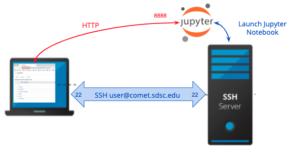
Note: google chrome has many local ports open in the range of 7713 - 7794. They are all connect to 80 or 443 on the other end.

3. Log onto comet.sdsc.edu

ssh -Y -l <username> <system name>.sdsc.edu

create a test directory, or cd into one you have already created
Clone the examples repository:

git clone https://github.com/sdsc-hpc-training-org/notebook-examples.git

Run the jupyter command. Be sure to set the –ip to use the hostname, which will appear in your URL :

[mthomas@comet-14-01:~] jupyter notebook  --no-browser --ip=`/bin/hostname`

You will see output similar to that shown below:

[I 08:06:32.961 NotebookApp] JupyterLab extension loaded from /home/mthomas/miniconda3/lib/python3.7/site-packages/jupyterlab
[I 08:06:32.961 NotebookApp] JupyterLab application directory is /home/mthomas/miniconda3/share/jupyter/lab
[I 08:06:33.486 NotebookApp] Serving notebooks from local directory: /home/mthomas
[I 08:06:33.487 NotebookApp] The Jupyter Notebook is running at:
[I 08:06:33.487 NotebookApp] http://comet-14-01.sdsc.edu:8888/?token=6d7a48dda7cc1635d6d08f63aa1a696008fa89d8aa84ad2b
[I 08:06:33.487 NotebookApp]  or http://127.0.0.1:8888/?token=6d7a48dda7cc1635d6d08f63aa1a696008fa89d8aa84ad2b
[I 08:06:33.487 NotebookApp] Use Control-C to stop this server and shut down all kernels (twice to skip confirmation).
[C 08:06:33.494 NotebookApp]

    To access the notebook, open this file in a browser:
        file:///home/mthomas/.local/share/jupyter/runtime/nbserver-6614-open.html
    Or copy and paste one of these URLs:
        http://comet-14-01.sdsc.edu:8888/?token=6d7a48dda7cc1635d6d08f63aa1a696008fa89d8aa84ad2b
     or http://127.0.0.1:8888/?token=6d7a48dda7cc1635d6d08f63aa1a696008fa89d8aa84ad2b
[I 08:06:45.773 NotebookApp] 302 GET /?token=6d7a48dda7cc1635d6d08f63aa1a696008fa89d8aa84ad2b (76.176.117.51) 0.74ms
[E 08:06:45.925 NotebookApp] Could not open static file ''
[W 08:06:46.033 NotebookApp] 404 GET /static/components/react/react-dom.production.min.js (76.176.117.51) 7.39ms referer=http://comet-14-01.sdsc.edu:8888/tree?token=6d7a48dda7cc1635d6d08f63aa1a696008fa89d8aa84ad2b
[W 08:06:46.131 NotebookApp] 404 GET /static/components/react/react-dom.production.min.js (76.176.117.51) 1.02ms referer=http://comet-14-01.sdsc.edu:8888/tree?token=6d7a48dda7cc1635d6d08f63aa1a696008fa89d8aa84ad2b

Notice that the notebook URL is using HTTP, and when you connect the browser on your local sysetm to this URL, the connection will not be secure. Note: it is against SDSC Comet policy to run applications on the login nodes, and any applications being run will be killed by the system admins. A better way is to run the jobs on an interactive node or on a compute node using the batch queue (see the Comet User Guide), or on a compute node, which is described in the next sections.

5. Obtain an interactive node

Jobs can be run on the cluster in batch mode or in interactive mode. Batch jobs are performed remotely and without manual intervention. Interactive mode enable you to run/compile your program and environment setup on a compute node dedicated to you. To obtain an interactive node, type:

srun --pty --nodes=1 --ntasks-per-node=24 -p compute -t 02:00:00 --wait 0 /bin/bash

You will have to wait for your node to be allocated - which can take a few or many minutes. You will see pending messages like the ones below:

srun: job 24000544 queued and waiting for resources
srun: job 24000544 has been allocated resources
[mthomas@comet-18-29:~/hpctrain/python/PythonSeries]

You can also check the status of jobs in the queue system to get an idea of how long you may need to wait.

Launch the Jupyter Notebook application. Note: this application will be running on comet, and you will be given a URL which will connect your local web browser the interactive comet session:

jupyter notebook --no-browser --ip=`/bin/hostname`

This will give you an address which has localhost in it and a token. Something like:

http://comet-14-0-4:8888/?token=xxxxxxxxxxxxxxxxxxxxxxxxxxxxxxxxxxxxxxxxxx

You can then paste it into your browser. You will see a running Jupyter notebook and a listing of the notebooks in your directory. From there everything should be working as a regular notebook. Note: This token is your auth so don’t email/send it around. It will go away when you stop the notebook.

To learn about Python, run the Python basics.ipynb notebook. To see an example of remote visualization, run the Matplotlib.ipynb notebook!

5.1 Access the node in your browser

Copy the the URL above into the browser running on your laptop.

5.2 Use your jupyterlab/jupyter notebook server!

Enjoy. Note that your notebook is unsecured.

3.7 - AI-First Engeneering Cybertraining Spring 2021 - Module

Here you will find a number of modules and components for introducing you to AI-First Engineering

Big Data Applications are an important topic that have impact in academia and industry.

3.7.1 - 2021

Here you will find a number of modules and components for introducing you to AI-First Engineering.

Big Data Applications are an important topic that have impact in academia and industry.

3.7.1.1 - Introduction to AI-Driven Digital Transformation

Last Semester’s Introductory Lecture with introduction to and Motivation for Big Data Applications and Analytics Class. See section G for material directly related to this lass but all sections are relevant

This Lecture is recorded in 8 parts and gives an introduction and motivation for the class. This and other lectures in class are divided into “bite-sized lessons” from 5 to 30 minutes in length; that’s why it has 8 parts.

Lecture explains what students might gain from the class even if they end up with different types of jobs from data engineering, software engineering, data science or a business (application) expert. It stresses that we are well into a transformation that impacts industry research and the way life is lived. This transformation is centered on using the digital way with clouds, edge computing and deep learning giving the implementation. This “AI-Driven Digital Transformation” is as transformational as the Industrial Revolution in the past. We note that deep learning dominates most innovative AI replacing several traditional machine learning methods.

The slides for this course can be found at E534-Fall2020-Introduction

A: Getting Started: BDAA Course Introduction Part A: Big Data Applications and Analytics

This lesson describes briefly the trends driving and consequent of the AI-Driven Digital Transformation. It discusses the organizational aspects of the class and notes the two driving trends are clouds and AI. Clouds are mature and a dominant presence. AI is still rapidly changing and we can expect further major changes. The edge (devices and associated local fog computing) has always been important but now more is being done there.

B: Technology Futures from Gartner’s Analysis: BDAA Course Introduction Part B: Big Data Applications and Analytics

This lesson goes through the technologies (AI Edge Cloud) from 2008-2020 that are driving the AI-Driven Digital Transformation. we use Hype Cycles and Priority Matrices from Gartner tracking importance concepts from the Innovation Trigger, Peak of Inflated Expectations through the Plateau of Productivity. We contrast clouds and AI.

C: Big Data Trends: BDAA Course Introduction Part C: Big Data Applications and Analytics

This gives illustrations of sources of big data.
It gives key graphs of data sizes, images uploaded; computing, data, bandwidth trends;
Cloud-Edge architecture.
Intelligent machines and comparison of data from aircraft engine monitors compared to Twitter

D: Computing Trends: BDAA Course Introduction Part D: Big Data Applications and Analytics

Multicore revolution
Overall Global AI and Modeling Supercomputer GAIMSC
Moores Law compared to Deep Learning computing needs
Intel and NVIDIA status

E: Big Data and Science: BDAA Course Introduction Part E: Big Data Applications and Analytics

Applications and Analytics
Cyberinfrastructure, e-moreorlessanything.
LHC, Higgs Boson and accelerators.
Astronomy, SKA, multi-wavelength.
Polar Grid.
Genome Sequencing.
Examples, Long Tail of Science.
Wired’s End of Science; the 4 paradigms.
More data versus Better algorithms.

F: Big Data Systems: BDAA Course Introduction Part F: Big Data Applications and Analytics

Clouds, Service-oriented architectures, HPC High Performance Computing, Apace Software
DIKW process illustrated by Google maps
Raw data to Information/Knowledge/Wisdom/Decision Deluge from the EdgeInformation/Knowledge/Wisdom/Decision Deluge
Parallel Computing
Map Reduce

G: Industry Transformation: BDAA Course Introduction Part G: Big Data Applications and Analytics

AI grows in importance and industries transform with

Core Technologies related to
New “Industries” over the last 25 years
Traditional “Industries” Transformed; malls and other old industries transform
Good to be master of Cloud Computing and Deep Learning
AI-First Industries,

H: Jobs and Conclusions: BDAA Course Introduction Part H: Big Data Applications and Analytics

Job trends
Become digitally savvy so you can take advantage of the AI/Cloud/Edge revolution with different jobs
The qualitative idea of Big Data has turned into a quantitative realization as Cloud, Edge and Deep Learning
Clouds are here to stay and one should plan on exploiting them
Data Intensive studies in business and research continue to grow in importance

3.7.1.2 - AI-First Engineering Cybertraining Spring 2021

Updated On an ongoing Basis

This describes weekly meeting and overall videos and homeworks

Contents

Week 1

Lecture

Our first meeting is 01:10P-02:25P on Tuesday

The zoom will be https://iu.zoom.us/my/gc.fox

We will discuss how to interact with us. We can adjust the course somewhat.

Also as lectures are/will be put on YouTube, we will go to one lecture per week – we will choose day

The Syllabus has a general course description

Please communicate initially by email gcf@iu.edu

This first class discussed structure of class and agreed to have a section on deep learning technology.

We gave Introductory Lecture

Assignments

Assignment Github: Get a github.com account
Assignment Slack: Enroll in our slack at * https://join.slack.com/t/cybertraining-3bz7942/shared_invite/zt-kzs969ea-x35oX9wdjspX7NmkpSfUpw Post your github account name into the slack channel #general and #ai
Post a 2-3 paragraph formal Bio (see IEEE papers what a formal bio is. Use google to find examples for Bios or look at Geoffreys or Gregors Web Pages.)

Week 2

Introduction

We gave an introductory lecture to optimization and deep learning. Unfortunately we didn’t record the zoom serssion but we did make an offline recording with slides IntroDLOpt: Introduction to Deep Learning and Optimization and YouTube

Google Colab

We also went through material on using Google Colab with examples. This is a lecture plus four Python notebooks

with recorded video

First DL: Deep Learning MNIST Example Spring 2021

We now have recorded all the introductory deep learning material

with recorded videos

IntroDLOpt: Introduction to Deep Learning and Optimization

Video: IntroDLOpt: Introduction to Deep Learning and Optimization

Opt: Overview of Optimization Spring2021

Video: Opt: Overview of Optimization Spring2021

DLBasic: Deep Learning - Some examples Spring 2021

Video: DLBasic: Deep Learning - Some examples Spring 2021

DLBasic: Components of Deep Learning Systems

Video: DLBasic: Components of Deep Learning Systems

DLBasic: Summary of Types of Deep Learning Systems

Video: DLBasic: Summary of Types of Deep Learning Systems

Week 3

Deep Learning Examples, 1

We discussed deep learning examples covering first half of slides DLBasic: Deep Learning - Some examples with recorded video

Week 4

Deep Learning Examples, 2 plus Components

We concluded deep learning examples and covered components with slides Deep Learning: More Examples and Components with recorded video

Week 5

Deep Learning Networks plus Overview of Optimization

We covered two topics in this weeks video

Deep Learning Networks with presentation DLBasic: Types of Deep Learning Networks: Summary
General Issues in Optimization with presentation Week5 Presentation on Optimization

with recorded video

Week 6

Deep Learning and AI Examples in Health and Medicine

We went about 2/3rds of way through presentation AI First Scenarios: Health and Medicine

with recorded video

Week 7

Deep Learning and AI Examples

We finished the last 1/3rd of the presentation AI First Scenarios: Health and Medicine
We finished AI First Scenarios - Space
We started AI First Scenarios - Energy

with recorded video

Week 8

Deep Learning and AI Examples

We finished AI First Scenarios - Energy
We started AI First Scenarios: Banking and FinTech

with recorded video

Week 9

Deep Learning and AI Examples

We ended AI First Scenarios: Banking and FinTech
We started AI Scenarios in Mobility and Transportation Systems

with recorded video

Week 10

GitHub for the Class project

We explain how to use GitHub for the class project. A video is available on YouTube. Please note that we only uploaded the relevant portion. The other half of the lecture went into individual comments for each student which we have not published. The comments are included in the GitHub repository.

Note project guidelines are given here

Video

Week 11

The Final Project

We described the gidelines of final projects in Slides
We were impressed by the seven student presentations describing their chosen project and approach.

Video

Week 12

Practical Issues in Deep Learning for Earthquakes

We used our research on Earthquake forecasting, to illustrate deep learning for Time Series with slides

Video

Week 13

Practical Issues in Deep Learning for Earthquakes

We continued discussion that illustrated deep learning for Time Series with the same slides as last week

Video

3.7.1.3 - Introduction to AI in Health and Medicine

This section discusses the health and medicine sector

Overview

This module discusses AI and the digital transformation for the Health and Medicine Area with a special emphasis on COVID-19 issues. We cover both the impact of COVID and some of the many activities that are addressing it. Parts B and C have an extensive general discussion of AI in Health and Medicine

The complete presentation is available at Google Slides while the videos are a YouTube playlist

Part A: Introduction

This lesson describes some overarching issues including the

Summary in terms of Hypecycles
Players in the digital health ecosystem and in particular role of Big Tech which has needed AI expertise and infrastructure from clouds to smart watches/phones
Views of Pataients and Doctors on New Technology
Role of clouds. This is essentially assumed throughout presentation but not stressed.
Importance of Security
Introduction to Internet of Medical Things; this area is discussed in more detail later in preserntation

slides

Part B: Diagnostics

This highlights some diagnostic appliocations of AI and the digital transformation. Part C also has some diagnostic coverage – especially particular applications

General use of AI in Diagnostics
Early progress in diagnostic imaging including Radiology and Opthalmology
AI In Clinical Decision Support
Digital Therapeutics is a recognized and growing activity area

slides

Part C: Examples

This lesson covers a broad range of AI uses in Health and Medicine

Flagging Issues requirng urgent attentation and more generally AI for Precision Merdicine
Oncology and cancer have made early progress as exploit AI for images. Avoiding mistakes and diagnosing curable cervical cancer in developing countries with less screening.
Predicting Gestational Diabetes
cardiovascular diagnostics and AI to interpret and guide Ultrasound measurements
Robot Nurses and robots to comfort patients
AI to guide cosmetic surgery measuring beauty
AI in analysis DNA in blood tests
AI For Stroke detection (large vessel occlusion)
AI monitoring of breathing to flag opioid-induced respiratory depression.
AI to relieve administration burden including voice to text for Doctor’s notes
AI in consumer genomics
Areas that are slow including genomics, Consumer Robotics, Augmented/Virtual Reality and Blockchain
AI analysis of information resources flags probleme earlier
Internet of Medical Things applications from watches to toothbrushes

slides

Part D: Impact of Covid-19

This covers some aspects of the impact of COVID -19 pandedmic starting in March 2020

The features of the first stimulus bill
Impact on Digital Health, Banking, Fintech, Commerce – bricks and mortar, e-commerce, groceries, credit cards, advertising, connectivity, tech industry, Ride Hailing and Delivery,
Impact on Restaurants, Airlines, Cruise lines, general travel, Food Delivery
Impact of working from home and videoconferencing
The economy and
The often positive trends for Tech industry

slides

Part E: Covid-19 and Recession

This is largely outdated as centered on start of pandemic induced recession. and we know what really happenmed now. Probably the pandemic accelerated the transformation of industry and the use of AI.

slides

Part F: Tackling Covid-19

This discusses some of AI and digital methods used to understand and reduce impact of COVID-19

Robots for remote patient examination
computerized tomography scan + AI to identify COVID-19
Early activities of Big Tech and COVID
Other early biotech activities with COVID-19
Remote-work technology: Hopin, Zoom, Run the World, FreeConferenceCall, Slack, GroWrk, Webex, Lifesize, Google Meet, Teams
Vaccines
Wearables and Monitoring, Remote patient monitoring
Telehealth, Telemedicine and Mobile Health

slides

Part G: Data and Computational Science and Covid-19

This lesson reviews some sophisticated high performance computing HPC and Big Data approaches to COVID

Rosetta volunteer computer to analyze proteins
COVID-19 High Performance Computing Consortium
AI based drug discovery by startup Insilico Medicine
Review of several research projects
Global Pervasive Computational Epidemiology for COVID-19 studies
Simulations of Virtual Tissues at Indiana University available on nanoHUB

slides

Part H: Screening Drug and Candidates

A major project involving Department of Energy Supercomputers

General Structure of Drug Discovery
DeepDriveMD Project using AI combined with molecular dynamics to accelerate discovery of drug properties

slides

Part I: Areas for Covid19 Study and Pandemics as Complex Systems

slides

Possible Projects in AI for Health and Medicine and especially COVID-19
Pandemics as a Complex System
AI and computational Futures for Complex Systems

3.7.1.4 - Mobility (Industry)

This section discusses the mobility in Industry

Overview

Industry being transformed by a) Autonomy (AI) and b) Electric power
Established Organizations can’t change
- General Motors (employees: 225,000 in 2016 to around 180,000 in 2018) finds it hard to compete with Tesla (42000 employees)
- Market value GM was half the market value of Tesla at the start of 2020 but is now just 11% October 2020
- GM purchased Cruise to compete
- Funding and then buying startups is an important “transformation” strategy
Autonomy needs Sensors Computers Algorithms and Software
- Also experience (training data)
- Algorithms main bottleneck; others will automatically improve although lots of interesting work in new sensors, computers and software
- Over the last 3 years, electrical power has gone from interesting to “bound to happen”; Tesla’s happy customers probably contribute to this
- Batteries and Charging stations needed

Summary Slides

Full Slide Deck

Mobility Industry A: Introduction

Futures of Automobile Industry, Mobility, and Ride-Hailing
Self-cleaning cars
Medical Transportation
Society of Automotive Engineers, Levels 0-5
Gartner’s conservative View

Mobility Industry B: Self Driving AI

Image processing and Deep Learning
Examples of Self Driving cars
Road construction Industry
Role of Simulated data
Role of AI in autonomy
Fleet cars
3 Leaders: Waymo, Cruise, NVIDIA

Mobility Industry C: General Motors View

Talk by Dave Brooks at GM, “AI for Automotive Engineering”
Zero crashes, zero emission, zero congestion
GM moving to electric autonomous vehicles

Mobility Industry D: Self Driving Snippets

Worries about and data on its Progress
Tesla’s specialized self-driving chip
Some tasks that are hard for AI
Scooters and Bikes

Mobility Industry E: Electrical Power

Rise in use of electrical power
Special opportunities in e-Trucks and time scale
Future of Trucks
Tesla market value
Drones and Robot deliveries; role of 5G
Robots in Logistics

3.7.1.5 - Space and Energy

This section discusses the space and energy.

Overview

Energy sources and AI for powering Grids.
Energy Solution from Bill Gates
Space and AI

Full Slide Deck

A: Energy

Distributed Energy Resources as a grid of renewables with a hierarchical set of Local Distribution Areas
Electric Vehicles in Grid
Economics of microgrids
Investment into Clean Energy
Batteries
Fusion and Deep Learning for plasma stability
AI for Power Grid, Virtual Power Plant, Power Consumption Monitoring, Electricity Trading

Slides

B: Clean Energy startups from Bill Gates

26 Startups in areas like long-duration storage, nuclear energy, carbon capture, batteries, fusion, and hydropower …
The slide deck gives links to 26 companies from their website and pitchbook which describes their startup status (#employees, funding)
It summarizes their products

Slides

C: Space

Space supports AI with communications, image data and global navigation
AI Supports space in AI-controlled remote manufacturing, imaging control, system control, dynamic spectrum use
Privatization of Space - SpaceX, Investment
57,000 satellites through 2029

Slides

3.7.1.6 - AI In Banking

This section discusses AI in Banking

Overview

In this lecture, AI in Banking is discussed. Here we focus on the transition of legacy banks towards AI based banking, real world examples of AI in Banking, banking systems and banking as a service.

Slides

AI in Banking A: The Transition of legacy Banks

Types of AI that is used
Closing of physical branches
Making the transition
Growth in Fintech as legacy bank services decline

AI in Banking B: FinTech

Fintech examples and investment
Broad areas of finance/banking where Fintech operating

AI in Banking C: Neobanks

Types and Examples of neobanks
Customer uptake by world region
Neobanking in Small and Medium Business segment
Neobanking in real estate, mortgages
South American Examples

AI in Banking D: The System

The Front, Middle, Back Office
Front Office: Chatbots
Robo-advisors
Middle Office: Fraud, Money laundering
Fintech
Payment Gateways (Back Office)
Banking as a Service

AI in Banking E: Examples

Credit cards
The stock trading ecosystem
Robots counting coins
AI in Insurance: Chatbots, Customer Support
Banking itself
Handwriting recognition
Detect leaks for insurance

AI in Banking F: As a Service

Banking Services Stack
Business Model
Several Examples
Metrics compared among examples
Breadth, Depth, Reputation, Speed to Market, Scalability

3.7.1.7 - Cloud Computing

Cloud Computing

E534 Cloud Computing Unit

Full Slide Deck

Overall Summary

Video:

Defining Clouds I: Basic definition of cloud and two very simple examples of why virtualization is important

How clouds are situated wrt HPC and supercomputers
Why multicore chips are important
Typical data center

Video:

Defining Clouds II: Service-oriented architectures: Software services as Message-linked computing capabilities

The different aaS’s: Network, Infrastructure, Platform, Software
The amazing services that Amazon AWS and Microsoft Azure have
Initial Gartner comments on clouds (they are now the norm) and evolution of servers; serverless and microservices
Gartner hypecycle and priority matrix on Infrastructure Strategies

Video:

How important are they?
How much money do they make?

Video:

Virtualization: Virtualization Technologies, Hypervisors and the different approaches

KVM Xen, Docker and Openstack

Video:

Cloud Infrastructure I: Comments on trends in the data center and its technologies

Clouds physically across the world
Green computing
Fraction of world’s computing ecosystem in clouds and associated sizes
An analysis from Cisco of size of cloud computing

Video:

Cloud Infrastructure II: Gartner hypecycle and priority matrix on Compute Infrastructure

Containers compared to virtual machines
The emergence of artificial intelligence as a dominant force

Video:

Cloud Software: HPC-ABDS with over 350 software packages and how to use each of 21 layers

Google’s software innovations
MapReduce in pictures
Cloud and HPC software stacks compared
Components need to support cloud/distributed system programming

Video:

Cloud Applications I: Clouds in science where area called cyberinfrastructure; the science usage pattern from NIST

Artificial Intelligence from Gartner

Video:

Cloud Applications II: Characterize Applications using NIST approach

Internet of Things
Different types of MapReduce

Video:

Parallel Computing Analogies: Parallel Computing in pictures

Some useful analogies and principles

Video:

Real Parallel Computing: Single Program/Instruction Multiple Data SIMD SPMD

Big Data and Simulations Compared
What is hard to do?

Video:

Storage: Cloud data approaches

Repositories, File Systems, Data lakes

Video:

HPC and Clouds: The Branscomb Pyramid

Supercomputers versus clouds
Science Computing Environments

Video:

Comparison of Data Analytics with Simulation: Structure of different applications for simulations and Big Data

Software implications
Languages

Video:

The Future I: The Future I: Gartner cloud computing hypecycle and priority matrix 2017 and 2019

Hyperscale computing
Serverless and FaaS
Cloud Native
Microservices
Update to 2019 Hypecycle

Video:

Future and Other Issues II: Security

Blockchain

Video:

Future and Other Issues III: Fault Tolerance

Video:

3.7.1.8 - Transportation Systems

This section discusses the transportation systems

Transportation Systems Summary

The ride-hailing industry highlights the growth of a new “Transportation System” TS a. For ride-hailing TS controls rides matching drivers and customers; it predicts how to position cars and how to avoid traffic slowdowns b. However, TS is much bigger outside ride-hailing as we move into the “connected vehicle” era c. TS will probably find autonomous vehicles easier to deal with than human drivers
Cloud Fog and Edge components
Autonomous AI was centered on generalized image processing
TS also needs AI (and DL) but this is for routing and geospatial time-series; different technologies from those for image processing

Slides

Transportation Systems A: Introduction

“Smart” Insurance
Fundamentals of Ride-Hailing

Transportation Systems B: Components of a Ride-Hailing System

Transportation Brain and Services
Maps, Routing,
Traffic forecasting with deep learning

Transportation Systems C: Different AI Approaches in Ride-Hailing

View as a Time Series: LSTM and ARIMA
View as an image in a 2D earth surface - Convolutional networks
Use of Graph Neural Nets
Use of Convolutional Recurrent Neural Nets
Spatio-temporal modeling
Comparison of data with predictions
Reinforcement Learning
Formulation of General Geospatial Time-Series Problem

3.7.1.9 - Commerce

This section discusses Commerce

Overview

Slides

AI in Commerce A: The Old way of doing things

AI in Commerce
AI-First Engineering, Deep Learning
E-commerce and the transformation of “Bricks and Mortar”

AI in Commerce B: AI in Retail

Personalization
Search
Image Processing to Speed up Shopping
Walmart

AI in Commerce C: The Revolution that is Amazon

Retail Revolution
Saves Time, Effort and Novelity with Modernized Retail
Looking ahead of Retail evolution

AI in Commerce D: DLMalls e-commerce

Amazon sellers
Rise of Shopify
Selling Products on Amazon

AI in Commerce E: Recommender Engines, Digital media

Spotify recommender engines
Collaborative Filtering
Audio Modelling
DNN for Recommender engines

3.7.1.10 - Python Warm Up

Python Exercise on Google Colab

View in Github

Download Notebook

In this exercise, we will take a look at some basic Python Concepts needed for day-to-day coding.

Check the installed Python version.

! python --version

Python 3.7.6

Simple For Loop

for i in range(10):
  print(i)

List

list_items = ['a', 'b', 'c', 'd', 'e']

Retrieving an Element

list_items[2]

'c'

Append New Values

list_items.append('f')

list_items

['a', 'b', 'c', 'd', 'e', 'f']

Remove an Element

list_items.remove('a')

list_items

['b', 'c', 'd', 'e', 'f']

Dictionary

dictionary_items = {'a':1, 'b': 2, 'c': 3}

Retrieving an Item by Key

dictionary_items['b']

Append New Item with Key

dictionary_items['c'] = 4

dictionary_items

{'a': 1, 'b': 2, 'c': 4}

Delete an Item with Key

del dictionary_items['a']

dictionary_items

{'b': 2, 'c': 4}

Comparators

x = 10
y = 20 
z = 30

x > y

False

x < z

True

z == x

False

if x < z:
  print("This is True")

This is True

if x > z:
  print("This is True")
else:
  print("This is False")

This is False

Arithmetic

k = x * y * z
k

j = x + y + z
j

m = x -y 
m

-10

n = x / z
n

0.3333333333333333

Numpy

Create a Random Numpy Array

import numpy as np

a = np.random.rand(100)
a.shape

(100,)

Reshape Numpy Array

b = a.reshape(10,10)
b.shape

(10, 10)

Manipulate Array Elements

c = b * 10
c[0]

array([3.33575458, 7.39029235, 5.54086921, 9.88592471, 4.9246252 ,
       1.76107178, 3.5817523 , 3.74828708, 3.57490794, 6.55752319])

c = np.mean(b,axis=1)
c.shape

print(c)

[0.60673061 0.4223565  0.42687517 0.6260857  0.60814217 0.66445627 
  0.54888432 0.68262262 0.42523459 0.61504903]

3.7.1.11 - Distributed Training for MNIST

Distributed Training for MNIST

View in Github

Download Notebook

In this lesson we discuss in how to create a simple IPython Notebook to solve an image classification problem with Multi Layer Perceptron with LSTM.

Pre-requisites

Install the following Python packages

cloudmesh-installer
cloudmesh-common

pip3 install cloudmesh-installer
pip3 install cloudmesh-common

Sample MLP + LSTM with Tensorflow Keras

Import Libraries

from __future__ import absolute_import
from __future__ import division
from __future__ import print_function

import numpy as np
import tensorflow as tf
from tensorflow.keras.models import Sequential
from tensorflow.keras.layers import Dense, Activation, SimpleRNN, InputLayer, LSTM, Dropout
from tensorflow.keras.utils import to_categorical, plot_model
from tensorflow.keras.datasets import mnist
from cloudmesh.common.StopWatch import StopWatch

Download Data and Pre-Process

StopWatch.start("data-load")
(x_train, y_train), (x_test, y_test) = mnist.load_data()
StopWatch.stop("data-load")


StopWatch.start("data-pre-process")
num_labels = len(np.unique(y_train))


y_train = to_categorical(y_train)
y_test = to_categorical(y_test)


image_size = x_train.shape[1]
x_train = np.reshape(x_train,[-1, image_size, image_size])
x_test = np.reshape(x_test,[-1, image_size, image_size])
x_train = x_train.astype('float32') / 255
x_test = x_test.astype('float32') / 255
StopWatch.stop("data-pre-process")

input_shape = (image_size, image_size)
batch_size = 128
units = 256
dropout = 0.2

Define Model

Here we use the Tensorflow distributed training components to train the model in multiple CPUs or GPUs. In the Colab instance multiple GPUs are not supported. Hence, the training must be done in the device type ‘None’ when selecting the ‘runtime type’ from Runtime menu. To run with multiple-GPUs no code change is required. Learn more about distributed training.

StopWatch.start("compile")
strategy = tf.distribute.MirroredStrategy()
with strategy.scope():
  model = Sequential()
  # LSTM Layers
  model.add(LSTM(units=units,                      
                      input_shape=input_shape,
                      return_sequences=True))
  model.add(LSTM(units=units, 
                      dropout=dropout,                      
                      return_sequences=True))
  model.add(LSTM(units=units, 
                      dropout=dropout,                      
                      return_sequences=False))
  # MLP Layers
  model.add(Dense(units))
  model.add(Activation('relu'))
  model.add(Dropout(dropout))
  model.add(Dense(units))
  model.add(Activation('relu'))
  model.add(Dropout(dropout))
  # Softmax_layer
  model.add(Dense(num_labels))
  model.add(Activation('softmax'))
  model.summary()
  plot_model(model, to_file='rnn-mnist.png', show_shapes=True)
  
  print("Number of devices: {}".format(strategy.num_replicas_in_sync))

  model.compile(loss='categorical_crossentropy',
                optimizer='sgd',
                metrics=['accuracy'])
StopWatch.stop("compile")

Model: "sequential_2"
_________________________________________________________________
Layer (type)                 Output Shape              Param #   
=================================================================
lstm_6 (LSTM)                (None, 28, 256)           291840    
_________________________________________________________________
lstm_7 (LSTM)                (None, 28, 256)           525312    
_________________________________________________________________
lstm_8 (LSTM)                (None, 256)               525312    
_________________________________________________________________
dense_6 (Dense)              (None, 256)               65792     
_________________________________________________________________
activation_6 (Activation)    (None, 256)               0         
_________________________________________________________________
dropout_4 (Dropout)          (None, 256)               0         
_________________________________________________________________
dense_7 (Dense)              (None, 256)               65792     
_________________________________________________________________
activation_7 (Activation)    (None, 256)               0         
_________________________________________________________________
dropout_5 (Dropout)          (None, 256)               0         
_________________________________________________________________
dense_8 (Dense)              (None, 10)                2570      
_________________________________________________________________
activation_8 (Activation)    (None, 10)                0         
=================================================================
Total params: 1,476,618
Trainable params: 1,476,618
Non-trainable params: 0
_________________________________________________________________
INFO:tensorflow:Using MirroredStrategy with devices ('/job:localhost/replica:0/task:0/device:GPU:0',)
Number of devices: 1
INFO:tensorflow:Reduce to /job:localhost/replica:0/task:0/device:CPU:0 then broadcast to ('/job:localhost/replica:0/task:0/device:CPU:0',).
INFO:tensorflow:Reduce to /job:localhost/replica:0/task:0/device:CPU:0 then broadcast to ('/job:localhost/replica:0/task:0/device:CPU:0',).
INFO:tensorflow:Reduce to /job:localhost/replica:0/task:0/device:CPU:0 then broadcast to ('/job:localhost/replica:0/task:0/device:CPU:0',).
INFO:tensorflow:Reduce to /job:localhost/replica:0/task:0/device:CPU:0 then broadcast to ('/job:localhost/replica:0/task:0/device:CPU:0',).

Train

StopWatch.start("train")
model.fit(x_train, y_train, epochs=30, batch_size=batch_size)
StopWatch.stop("train")

Epoch 1/30
469/469 [==============================] - 7s 16ms/step - loss: 2.0427 - accuracy: 0.2718
Epoch 2/30
469/469 [==============================] - 7s 16ms/step - loss: 1.6934 - accuracy: 0.4007
Epoch 3/30
469/469 [==============================] - 7s 16ms/step - loss: 1.2997 - accuracy: 0.5497
...
Epoch 28/30
469/469 [==============================] - 8s 17ms/step - loss: 0.1175 - accuracy: 0.9640
Epoch 29/30
469/469 [==============================] - 8s 17ms/step - loss: 0.1158 - accuracy: 0.9645
Epoch 30/30
469/469 [==============================] - 8s 17ms/step - loss: 0.1098 - accuracy: 0.9661

Test

StopWatch.start("evaluate")
loss, acc = model.evaluate(x_test, y_test, batch_size=batch_size)
print("\nTest accuracy: %.1f%%" % (100.0 * acc))
StopWatch.stop("evaluate")

StopWatch.benchmark()

79/79 [==============================] - 3s 9ms/step - loss: 0.0898 - accuracy: 0.9719

Test accuracy: 97.2%

+---------------------+------------------------------------------------------------------+
| Attribute           | Value                                                            |
|---------------------+------------------------------------------------------------------|
| BUG_REPORT_URL      | "https://bugs.launchpad.net/ubuntu/"                             |
| DISTRIB_CODENAME    | bionic                                                           |
| DISTRIB_DESCRIPTION | "Ubuntu 18.04.5 LTS"                                             |
| DISTRIB_ID          | Ubuntu                                                           |
| DISTRIB_RELEASE     | 18.04                                                            |
| HOME_URL            | "https://www.ubuntu.com/"                                        |
| ID                  | ubuntu                                                           |
| ID_LIKE             | debian                                                           |
| NAME                | "Ubuntu"                                                         |
| PRETTY_NAME         | "Ubuntu 18.04.5 LTS"                                             |
| PRIVACY_POLICY_URL  | "https://www.ubuntu.com/legal/terms-and-policies/privacy-policy" |
| SUPPORT_URL         | "https://help.ubuntu.com/"                                       |
| UBUNTU_CODENAME     | bionic                                                           |
| VERSION             | "18.04.5 LTS (Bionic Beaver)"                                    |
| VERSION_CODENAME    | bionic                                                           |
| VERSION_ID          | "18.04"                                                          |
| cpu_count           | 2                                                                |
| mem.active          | 2.4 GiB                                                          |
| mem.available       | 10.3 GiB                                                         |
| mem.free            | 4.5 GiB                                                          |
| mem.inactive        | 5.4 GiB                                                          |
| mem.percent         | 18.6 %                                                           |
| mem.total           | 12.7 GiB                                                         |
| mem.used            | 3.3 GiB                                                          |
| platform.version    | #1 SMP Thu Jul 23 08:00:38 PDT 2020                              |
| python              | 3.7.10 (default, Feb 20 2021, 21:17:23)                          |
|                     | [GCC 7.5.0]                                                      |
| python.pip          | 19.3.1                                                           |
| python.version      | 3.7.10                                                           |
| sys.platform        | linux                                                            |
| uname.machine       | x86_64                                                           |
| uname.node          | b39e0899c1f8                                                     |
| uname.processor     | x86_64                                                           |
| uname.release       | 4.19.112+                                                        |
| uname.system        | Linux                                                            |
| uname.version       | #1 SMP Thu Jul 23 08:00:38 PDT 2020                              |
| user                | collab                                                           |
+---------------------+------------------------------------------------------------------+

+------------------+----------+---------+---------+---------------------+-------+--------------+--------+-------+-------------------------------------+
| Name             | Status   |    Time |     Sum | Start               | tag   | Node         | User   | OS    | Version                             |
|------------------+----------+---------+---------+---------------------+-------+--------------+--------+-------+-------------------------------------|
| data-load        | failed   |   0.473 |   0.473 | 2021-03-07 11:34:03 |       | b39e0899c1f8 | collab | Linux | #1 SMP Thu Jul 23 08:00:38 PDT 2020 |
| data-pre-process | failed   |   0.073 |   0.073 | 2021-03-07 11:34:03 |       | b39e0899c1f8 | collab | Linux | #1 SMP Thu Jul 23 08:00:38 PDT 2020 |
| compile          | failed   |   0.876 |   7.187 | 2021-03-07 11:38:05 |       | b39e0899c1f8 | collab | Linux | #1 SMP Thu Jul 23 08:00:38 PDT 2020 |
| train            | failed   | 229.341 | 257.023 | 2021-03-07 11:38:44 |       | b39e0899c1f8 | collab | Linux | #1 SMP Thu Jul 23 08:00:38 PDT 2020 |
| evaluate         | failed   |   2.659 |   4.25  | 2021-03-07 11:44:54 |       | b39e0899c1f8 | collab | Linux | #1 SMP Thu Jul 23 08:00:38 PDT 2020 |
+------------------+----------+---------+---------+---------------------+-------+--------------+--------+-------+-------------------------------------+

# csv,timer,status,time,sum,start,tag,uname.node,user,uname.system,platform.version
# csv,data-load,failed,0.473,0.473,2021-03-07 11:34:03,,b39e0899c1f8,collab,Linux,#1 SMP Thu Jul 23 08:00:38 PDT 2020
# csv,data-pre-process,failed,0.073,0.073,2021-03-07 11:34:03,,b39e0899c1f8,collab,Linux,#1 SMP Thu Jul 23 08:00:38 PDT 2020
# csv,compile,failed,0.876,7.187,2021-03-07 11:38:05,,b39e0899c1f8,collab,Linux,#1 SMP Thu Jul 23 08:00:38 PDT 2020
# csv,train,failed,229.341,257.023,2021-03-07 11:38:44,,b39e0899c1f8,collab,Linux,#1 SMP Thu Jul 23 08:00:38 PDT 2020
# csv,evaluate,failed,2.659,4.25,2021-03-07 11:44:54,,b39e0899c1f8,collab,Linux,#1 SMP Thu Jul 23 08:00:38 PDT 2020

Reference:

3.7.1.12 - MLP + LSTM with MNIST on Google Colab

MLP + LSTM with MNIST on Google Colab

View in Github

Download Notebook

In this lesson we discuss in how to create a simple IPython Notebook to solve an image classification problem with Multi Layer Perceptron with LSTM.

Pre-requisites

Install the following Python packages

cloudmesh-installer
cloudmesh-common

pip3 install cloudmesh-installer
pip3 install cloudmesh-common

Sample MLP + LSTM with Tensorflow Keras

Import Libraries

from __future__ import absolute_import
from __future__ import division
from __future__ import print_function

import numpy as np
import tensorflow as tf
from tensorflow.keras.models import Sequential
from tensorflow.keras.layers import Dense, Activation, SimpleRNN, InputLayer, LSTM, Dropout
from tensorflow.keras.utils import to_categorical, plot_model
from tensorflow.keras.datasets import mnist
from cloudmesh.common.StopWatch import StopWatch

Download Data and Pre-Process

StopWatch.start("data-load")
(x_train, y_train), (x_test, y_test) = mnist.load_data()
StopWatch.stop("data-load")


StopWatch.start("data-pre-process")
num_labels = len(np.unique(y_train))


y_train = to_categorical(y_train)
y_test = to_categorical(y_test)


image_size = x_train.shape[1]
x_train = np.reshape(x_train,[-1, image_size, image_size])
x_test = np.reshape(x_test,[-1, image_size, image_size])
x_train = x_train.astype('float32') / 255
x_test = x_test.astype('float32') / 255
StopWatch.stop("data-pre-process")

input_shape = (image_size, image_size)
batch_size = 128
units = 256
dropout = 0.2

Define Model

StopWatch.start("compile")
model = Sequential()
# LSTM Layers
model.add(LSTM(units=units,                      
                     input_shape=input_shape,
                     return_sequences=True))
model.add(LSTM(units=units, 
                     dropout=dropout,                      
                     return_sequences=True))
model.add(LSTM(units=units, 
                     dropout=dropout,                      
                     return_sequences=False))
# MLP Layers
model.add(Dense(units))
model.add(Activation('relu'))
model.add(Dropout(dropout))
model.add(Dense(units))
model.add(Activation('relu'))
model.add(Dropout(dropout))
# Softmax_layer
model.add(Dense(num_labels))
model.add(Activation('softmax'))
model.summary()
plot_model(model, to_file='rnn-mnist.png', show_shapes=True)


model.compile(loss='categorical_crossentropy',
              optimizer='sgd',
              metrics=['accuracy'])
StopWatch.stop("compile")

Model: "sequential"
_________________________________________________________________
Layer (type)                 Output Shape              Param #   
=================================================================
lstm (LSTM)                  (None, 28, 256)           291840    
_________________________________________________________________
lstm_1 (LSTM)                (None, 28, 256)           525312    
_________________________________________________________________
lstm_2 (LSTM)                (None, 256)               525312    
_________________________________________________________________
dense (Dense)                (None, 256)               65792     
_________________________________________________________________
activation (Activation)      (None, 256)               0         
_________________________________________________________________
dropout (Dropout)            (None, 256)               0         
_________________________________________________________________
dense_1 (Dense)              (None, 256)               65792     
_________________________________________________________________
activation_1 (Activation)    (None, 256)               0         
_________________________________________________________________
dropout_1 (Dropout)          (None, 256)               0         
_________________________________________________________________
dense_2 (Dense)              (None, 10)                2570      
_________________________________________________________________
activation_2 (Activation)    (None, 10)                0         
=================================================================
Total params: 1,476,618
Trainable params: 1,476,618
Non-trainable params: 0

Train

StopWatch.start("train")
model.fit(x_train, y_train, epochs=30, batch_size=batch_size)
StopWatch.stop("train")

469/469 [==============================] - 378s 796ms/step - loss: 2.2689 - accuracy: 0.2075

Test

StopWatch.start("evaluate")
loss, acc = model.evaluate(x_test, y_test, batch_size=batch_size)
print("\nTest accuracy: %.1f%%" % (100.0 * acc))
StopWatch.stop("evaluate")

StopWatch.benchmark()

79/79 [==============================] - 1s 7ms/step - loss: 2.2275 - accuracy: 0.3120

Test accuracy: 31.2%

+---------------------+------------------------------------------------------------------+
| Attribute           | Value                                                            |
|---------------------+------------------------------------------------------------------|
| BUG_REPORT_URL      | "https://bugs.launchpad.net/ubuntu/"                             |
| DISTRIB_CODENAME    | bionic                                                           |
| DISTRIB_DESCRIPTION | "Ubuntu 18.04.5 LTS"                                             |
| DISTRIB_ID          | Ubuntu                                                           |
| DISTRIB_RELEASE     | 18.04                                                            |
| HOME_URL            | "https://www.ubuntu.com/"                                        |
| ID                  | ubuntu                                                           |
| ID_LIKE             | debian                                                           |
| NAME                | "Ubuntu"                                                         |
| PRETTY_NAME         | "Ubuntu 18.04.5 LTS"                                             |
| PRIVACY_POLICY_URL  | "https://www.ubuntu.com/legal/terms-and-policies/privacy-policy" |
| SUPPORT_URL         | "https://help.ubuntu.com/"                                       |
| UBUNTU_CODENAME     | bionic                                                           |
| VERSION             | "18.04.5 LTS (Bionic Beaver)"                                    |
| VERSION_CODENAME    | bionic                                                           |
| VERSION_ID          | "18.04"                                                          |
| cpu_count           | 2                                                                |
| mem.active          | 1.9 GiB                                                          |
| mem.available       | 10.7 GiB                                                         |
| mem.free            | 7.3 GiB                                                          |
| mem.inactive        | 3.0 GiB                                                          |
| mem.percent         | 15.6 %                                                           |
| mem.total           | 12.7 GiB                                                         |
| mem.used            | 2.3 GiB                                                          |
| platform.version    | #1 SMP Thu Jul 23 08:00:38 PDT 2020                              |
| python              | 3.6.9 (default, Oct  8 2020, 12:12:24)                           |
|                     | [GCC 8.4.0]                                                      |
| python.pip          | 19.3.1                                                           |
| python.version      | 3.6.9                                                            |
| sys.platform        | linux                                                            |
| uname.machine       | x86_64                                                           |
| uname.node          | 9810ccb69d08                                                     |
| uname.processor     | x86_64                                                           |
| uname.release       | 4.19.112+                                                        |
| uname.system        | Linux                                                            |
| uname.version       | #1 SMP Thu Jul 23 08:00:38 PDT 2020                              |
| user                | collab                                                           |
+---------------------+------------------------------------------------------------------+

+------------------+----------+--------+--------+---------------------+-------+--------------+--------+-------+-------------------------------------+
| Name             | Status   |   Time |    Sum | Start               | tag   | Node         | User   | OS    | Version                             |
|------------------+----------+--------+--------+---------------------+-------+--------------+--------+-------+-------------------------------------|
| data-load        | failed   |  0.61  |  0.61  | 2021-02-21 21:35:06 |       | 9810ccb69d08 | collab | Linux | #1 SMP Thu Jul 23 08:00:38 PDT 2020 |
| data-pre-process | failed   |  0.076 |  0.076 | 2021-02-21 21:35:07 |       | 9810ccb69d08 | collab | Linux | #1 SMP Thu Jul 23 08:00:38 PDT 2020 |
| compile          | failed   |  6.445 |  6.445 | 2021-02-21 21:35:07 |       | 9810ccb69d08 | collab | Linux | #1 SMP Thu Jul 23 08:00:38 PDT 2020 |
| train            | failed   | 17.171 | 17.171 | 2021-02-21 21:35:13 |       | 9810ccb69d08 | collab | Linux | #1 SMP Thu Jul 23 08:00:38 PDT 2020 |
| evaluate         | failed   |  1.442 |  1.442 | 2021-02-21 21:35:31 |       | 9810ccb69d08 | collab | Linux | #1 SMP Thu Jul 23 08:00:38 PDT 2020 |
+------------------+----------+--------+--------+---------------------+-------+--------------+--------+-------+-------------------------------------+

# csv,timer,status,time,sum,start,tag,uname.node,user,uname.system,platform.version
# csv,data-load,failed,0.61,0.61,2021-02-21 21:35:06,,9810ccb69d08,collab,Linux,#1 SMP Thu Jul 23 08:00:38 PDT 2020
# csv,data-pre-process,failed,0.076,0.076,2021-02-21 21:35:07,,9810ccb69d08,collab,Linux,#1 SMP Thu Jul 23 08:00:38 PDT 2020
# csv,compile,failed,6.445,6.445,2021-02-21 21:35:07,,9810ccb69d08,collab,Linux,#1 SMP Thu Jul 23 08:00:38 PDT 2020
# csv,train,failed,17.171,17.171,2021-02-21 21:35:13,,9810ccb69d08,collab,Linux,#1 SMP Thu Jul 23 08:00:38 PDT 2020
# csv,evaluate,failed,1.442,1.442,2021-02-21 21:35:31,,9810ccb69d08,collab,Linux,#1 SMP Thu Jul 23 08:00:38 PDT 2020

Reference:

Orignal Source to Source Code

3.7.1.13 - MNIST Classification on Google Colab

MNIST Classification on Google Colab

View in Github

Download Notebook

In this lesson we discuss in how to create a simple IPython Notebook to solve an image classification problem. MNIST contains a set of pictures

Import Libraries

Note: https://python-future.org/quickstart.html

from __future__ import absolute_import
from __future__ import division
from __future__ import print_function

import numpy as np
from keras.models import Sequential
from keras.layers import Dense, Activation, Dropout
from keras.utils import to_categorical, plot_model
from keras.datasets import mnist

Warm Up Exercise

Pre-process data

Load data

First we load the data from the inbuilt mnist dataset from Keras Here we have to split the data set into training and testing data. The training data or testing data has two components. Training features and training labels. For instance every sample in the dataset has a corresponding label. In Mnist the training sample contains image data represented in terms of an array. The training labels are from 0-9.

Here we say x_train for training data features and y_train as the training labels. Same goes for testing data.

(x_train, y_train), (x_test, y_test) = mnist.load_data()

Downloading data from https://storage.googleapis.com/tensorflow/tf-keras-datasets/mnist.npz
11493376/11490434 [==============================] - 0s 0us/step

Identify Number of Classes

As this is a number classification problem. We need to know how many classes are there. So we’ll count the number of unique labels.

num_labels = len(np.unique(y_train))

Convert Labels To One-Hot Vector

Image Reshaping

The training model is designed by considering the data as a vector. This is a model dependent modification. Here we assume the image is a squared shape image.

image_size = x_train.shape[1]
input_size = image_size * image_size

Resize and Normalize

The next step is to continue the reshaping to a fit into a vector and normalize the data. Image values are from 0 - 255, so an easy way to normalize is to divide by the maximum value.

x_train = np.reshape(x_train, [-1, input_size])
x_train = x_train.astype('float32') / 255
x_test = np.reshape(x_test, [-1, input_size])
x_test = x_test.astype('float32') / 255

Create a Keras Model

Keras is a neural network library. The summary function provides tabular summary on the model you created. And the plot_model function provides a grpah on the network you created.

# Create Model
# network parameters
batch_size = 4
hidden_units = 64

model = Sequential()
model.add(Dense(hidden_units, input_dim=input_size))
model.add(Dense(num_labels))
model.add(Activation('softmax'))
model.summary()
plot_model(model, to_file='mlp-mnist.png', show_shapes=True)

Model: "sequential_1"
_________________________________________________________________
Layer (type)                 Output Shape              Param #   
=================================================================
dense_5 (Dense)              (None, 512)               401920    
_________________________________________________________________
dense_6 (Dense)              (None, 10)                5130      
_________________________________________________________________
activation_5 (Activation)    (None, 10)                0         
=================================================================
Total params: 407,050
Trainable params: 407,050
Non-trainable params: 0
_________________________________________________________________

images

Compile and Train

A keras model need to be compiled before it can be used to train the model. In the compile function, you can provide the optimization that you want to add, metrics you expect and the type of loss function you need to use.

Here we use adam optimizer, a famous optimizer used in neural networks.

The loss funtion we have used is the categorical_crossentropy.

Once the model is compiled, then the fit function is called upon passing the number of epochs, traing data and batch size.

The batch size determines the number of elements used per minibatch in optimizing the function.

Note: Change the number of epochs, batch size and see what happens.

model.compile(loss='categorical_crossentropy',
              optimizer='adam',
              metrics=['accuracy'])

model.fit(x_train, y_train, epochs=1, batch_size=batch_size)

469/469 [==============================] - 3s 7ms/step - loss: 0.3647 - accuracy: 0.8947





<tensorflow.python.keras.callbacks.History at 0x7fe88faf4c50>

Testing

Now we can test the trained model. Use the evaluate function by passing test data and batch size and the accuracy and the loss value can be retrieved.

MNIST_V1.0|Exercise: Try to observe the network behavior by changing the number of epochs, batch size and record the best accuracy that you can gain. Here you can record what happens when you change these values. Describe your observations in 50-100 words.

loss, acc = model.evaluate(x_test, y_test, batch_size=batch_size)
print("\nTest accuracy: %.1f%%" % (100.0 * acc))

79/79 [==============================] - 0s 4ms/step - loss: 0.2984 - accuracy: 0.9148

Test accuracy: 91.5%

Final Note

Homework

Solve Exercise MNIST_V1.0.

Reference:

Orignal Source to Source Code

3.7.1.14 - MNIST With PyTorch

MNIST With PyTorch

View in Github

Download Notebook

In this lesson we discuss in how to create a simple IPython Notebook to solve an image classification problem with Multi Layer Perceptron with PyTorch.

Import Libraries

import numpy as np
import torch
import torchvision
import matplotlib.pyplot as plt
from torchvision import datasets, transforms
from torch import nn
from torch import optim
from time import time
import os
from google.colab import drive

Pre-Process Data

Here we download the data using PyTorch data utils and transform the data by using a normalization function. PyTorch provides a data loader abstraction called a DataLoader where we can set the batch size, data shuffle per batch loading. Each data loader expecte a Pytorch Dataset. The DataSet abstraction and DataLoader usage can be found here

# Data transformation function 
transform = transforms.Compose([transforms.ToTensor(),
                              transforms.Normalize((0.5,), (0.5,)),
                              ])

# DataSet
train_data_set = datasets.MNIST('drive/My Drive/mnist/data/', download=True, train=True, transform=transform)
validation_data_set = datasets.MNIST('drive/My Drive/mnist/data/', download=True, train=False, transform=transform)

# DataLoader
train_loader = torch.utils.data.DataLoader(train_data_set, batch_size=32, shuffle=True)
validation_loader = torch.utils.data.DataLoader(validation_data_set, batch_size=32, shuffle=True)

Define Network

Here we select the matching input size compared to the network definition. Here data reshaping or layer reshaping must be done to match input data shape with the network input shape. Also we define a set of hidden unit sizes along with the output layers size. The output_size must match with the number of labels associated with the classification problem. The hidden units can be chosesn depending on the problem. nn.Sequential is one way to create the network. Here we stack a set of linear layers along with a softmax layer for the classification as the output layer.

input_size = 784
hidden_sizes = [128, 128, 64, 64]
output_size = 10

model = nn.Sequential(nn.Linear(input_size, hidden_sizes[0]),
                      nn.ReLU(),
                      nn.Linear(hidden_sizes[0], hidden_sizes[1]),
                      nn.ReLU(),
                      nn.Linear(hidden_sizes[1], hidden_sizes[2]),
                      nn.ReLU(),
                      nn.Linear(hidden_sizes[2], hidden_sizes[3]),
                      nn.ReLU(),
                      nn.Linear(hidden_sizes[3], output_size),
                      nn.LogSoftmax(dim=1))

                      
print(model)

Sequential(
  (0): Linear(in_features=784, out_features=128, bias=True)
  (1): ReLU()
  (2): Linear(in_features=128, out_features=128, bias=True)
  (3): ReLU()
  (4): Linear(in_features=128, out_features=64, bias=True)
  (5): ReLU()
  (6): Linear(in_features=64, out_features=64, bias=True)
  (7): ReLU()
  (8): Linear(in_features=64, out_features=10, bias=True)
  (9): LogSoftmax(dim=1)
)

Define Loss Function and Optimizer

Read more about Loss Functions and Optimizers supported by PyTorch.

criterion = nn.NLLLoss()
optimizer = optim.SGD(model.parameters(), lr=0.003, momentum=0.9)

Train

epochs = 5

for epoch in range(epochs):
    loss_per_epoch = 0
    for images, labels in train_loader:
        images = images.view(images.shape[0], -1)
    
        # Gradients cleared per batch
        optimizer.zero_grad()
        
        # Pass input to the model
        output = model(images)
        # Calculate loss after training compared to labels
        loss = criterion(output, labels)
        
        # backpropagation 
        loss.backward()
        
        # optimizer step to update the weights
        optimizer.step()
        
        loss_per_epoch += loss.item()
    average_loss = loss_per_epoch / len(train_loader)
    print("Epoch {} - Training loss: {}".format(epoch, average_loss))

Epoch 0 - Training loss: 1.3052690227402808
Epoch 1 - Training loss: 0.33809808635317695
Epoch 2 - Training loss: 0.22927882223685922
Epoch 3 - Training loss: 0.16807103878669521
Epoch 4 - Training loss: 0.1369301250545995

Model Evaluation

Similar to training data loader, we use the validation loader to load batch by batch and run the feed-forward network to get the expected prediction and compared to the label associated with the data point.

correct_predictions, all_count = 0, 0
# enumerate data from the data validation loader (loads a batch at a time)
for batch_id, (images,labels) in enumerate(validation_loader):
  for i in range(len(labels)):
    img = images[i].view(1, 784)
    # at prediction stage, only feed-forward calculation is required. 
    with torch.no_grad():
        logps = model(img)

    # Output layer of the network uses a LogSoftMax layer
    # Hence the probability must be calculated with the exponential values. 
    # The final layer returns an array of probabilities for each label
    # Pick the maximum probability and the corresponding index
    # The corresponding index is the predicted label 
    ps = torch.exp(logps)
    probab = list(ps.numpy()[0])
    pred_label = probab.index(max(probab))
    true_label = labels.numpy()[i]
    if(true_label == pred_label):
      correct_predictions += 1
    all_count += 1

print(f"Model Accuracy {(correct_predictions/all_count) * 100} %")

Model Accuracy 95.95 %

Reference:

3.7.1.15 - MNIST-AutoEncoder Classification on Google Colab

MNIST with AutoEncoder: Classification on Google Colab

View in Github

Download Notebook

Prerequisites

Install the following packages

! pip3 install cloudmesh-installer
! pip3 install cloudmesh-common

Import Libraries

import tensorflow as tf
from keras.layers import Dense, Input
from keras.layers import Conv2D, Flatten
from keras.layers import Reshape, Conv2DTranspose
from keras.models import Model
from keras.datasets import mnist
from keras.utils import plot_model
from keras import backend as K

import numpy as np
import matplotlib.pyplot as plt

Download Data and Pre-Process

(x_train, y_train), (x_test, y_test) = mnist.load_data()

image_size = x_train.shape[1]
x_train = np.reshape(x_train, [-1, image_size, image_size, 1])
x_test = np.reshape(x_test, [-1, image_size, image_size, 1])
x_train = x_train.astype('float32') / 255
x_test = x_test.astype('float32') / 255

input_shape = (image_size, image_size, 1)
batch_size = 32
kernel_size = 3
latent_dim = 16
hidden_units = [32, 64]

Downloading data from https://storage.googleapis.com/tensorflow/tf-keras-datasets/mnist.npz
11493376/11490434 [==============================] - 0s 0us/step

Define Model

inputs = Input(shape=input_shape, name='encoder_input')
x = inputs
x = Dense(hidden_units[0], activation='relu')(x)
x = Dense(hidden_units[1], activation='relu')(x)

shape = K.int_shape(x)

# generate latent vector
x = Flatten()(x)
latent = Dense(latent_dim, name='latent_vector')(x)

# instantiate encoder model
encoder = Model(inputs,
                latent,
                name='encoder')
encoder.summary()
plot_model(encoder,
           to_file='encoder.png',
           show_shapes=True)


latent_inputs = Input(shape=(latent_dim,), name='decoder_input')
x = Dense(shape[1] * shape[2] * shape[3])(latent_inputs)
x = Reshape((shape[1], shape[2], shape[3]))(x)
x = Dense(hidden_units[0], activation='relu')(x)
x = Dense(hidden_units[1], activation='relu')(x)

outputs = Dense(1, activation='relu')(x)

decoder = Model(latent_inputs, outputs, name='decoder')
decoder.summary()
plot_model(decoder, to_file='decoder.png', show_shapes=True)

autoencoder = Model(inputs,
                    decoder(encoder(inputs)),
                    name='autoencoder')
autoencoder.summary()
plot_model(autoencoder,
           to_file='autoencoder.png',
           show_shapes=True)

autoencoder.compile(loss='mse', optimizer='adam')

Model: "encoder"
_________________________________________________________________
Layer (type)                 Output Shape              Param #   
=================================================================
encoder_input (InputLayer)   [(None, 28, 28, 1)]       0         
_________________________________________________________________
dense_2 (Dense)              (None, 28, 28, 32)        64        
_________________________________________________________________
dense_3 (Dense)              (None, 28, 28, 64)        2112      
_________________________________________________________________
flatten_1 (Flatten)          (None, 50176)             0         
_________________________________________________________________
latent_vector (Dense)        (None, 16)                802832    
=================================================================
Total params: 805,008
Trainable params: 805,008
Non-trainable params: 0
_________________________________________________________________
Model: "decoder"
_________________________________________________________________
Layer (type)                 Output Shape              Param #   
=================================================================
decoder_input (InputLayer)   [(None, 16)]              0         
_________________________________________________________________
dense_4 (Dense)              (None, 50176)             852992    
_________________________________________________________________
reshape (Reshape)            (None, 28, 28, 64)        0         
_________________________________________________________________
dense_5 (Dense)              (None, 28, 28, 32)        2080      
_________________________________________________________________
dense_6 (Dense)              (None, 28, 28, 64)        2112      
_________________________________________________________________
dense_7 (Dense)              (None, 28, 28, 1)         65        
=================================================================
Total params: 857,249
Trainable params: 857,249
Non-trainable params: 0
_________________________________________________________________
Model: "autoencoder"
_________________________________________________________________
Layer (type)                 Output Shape              Param #   
=================================================================
encoder_input (InputLayer)   [(None, 28, 28, 1)]       0         
_________________________________________________________________
encoder (Functional)         (None, 16)                805008    
_________________________________________________________________
decoder (Functional)         (None, 28, 28, 1)         857249    
=================================================================
Total params: 1,662,257
Trainable params: 1,662,257
Non-trainable params: 0

Train

autoencoder.fit(x_train,
                x_train,
                validation_data=(x_test, x_test),
                epochs=1,
                batch_size=batch_size)

1875/1875 [==============================] - 112s 60ms/step - loss: 0.0268 - val_loss: 0.0131

<tensorflow.python.keras.callbacks.History at 0x7f3ecb2e0be0>

Test

x_decoded = autoencoder.predict(x_test)

79/79 [==============================] - 7s 80ms/step - loss: 0.2581 - accuracy: 0.9181

Test accuracy: 91.8%

Visualize

imgs = np.concatenate([x_test[:8], x_decoded[:8]])
imgs = imgs.reshape((4, 4, image_size, image_size))
imgs = np.vstack([np.hstack(i) for i in imgs])
plt.figure()
plt.axis('off')
plt.title('Input: 1st 2 rows, Decoded: last 2 rows')
plt.imshow(imgs, interpolation='none', cmap='gray')
plt.savefig('input_and_decoded.png')
plt.show()

3.7.1.16 - MNIST-CNN Classification on Google Colab

MNIST with Convolutional Neural Networks: Classification on Google Colab

View in Github

Download Notebook

Prerequisites

Install the following packages

! pip3 install cloudmesh-installer
! pip3 install cloudmesh-common

Import Libraries

from __future__ import absolute_import
from __future__ import division
from __future__ import print_function

import numpy as np
from keras.models import Sequential
from keras.layers import Activation, Dense, Dropout
from keras.layers import Conv2D, MaxPooling2D, Flatten, AveragePooling2D
from keras.utils import to_categorical, plot_model
from keras.datasets import mnist

Download Data and Pre-Process

(x_train, y_train), (x_test, y_test) = mnist.load_data()

num_labels = len(np.unique(y_train))

y_train = to_categorical(y_train)
y_test = to_categorical(y_test)

image_size = x_train.shape[1]
x_train = np.reshape(x_train,[-1, image_size, image_size, 1])
x_test = np.reshape(x_test,[-1, image_size, image_size, 1])
x_train = x_train.astype('float32') / 255
x_test = x_test.astype('float32') / 255

input_shape = (image_size, image_size, 1)
print(input_shape)
batch_size = 128
kernel_size = 3
pool_size = 2
filters = 64
dropout = 0.2

Downloading data from https://storage.googleapis.com/tensorflow/tf-keras-datasets/mnist.npz
11493376/11490434 [==============================] - 0s 0us/step
(28, 28, 1)

Define Model

model = Sequential()
model.add(Conv2D(filters=filters,
                 kernel_size=kernel_size,
                 activation='relu',
                 input_shape=input_shape,
                 padding='same'))
model.add(MaxPooling2D(pool_size))
model.add(Conv2D(filters=filters,
                 kernel_size=kernel_size,
                 activation='relu',
                 input_shape=input_shape,
                 padding='same'))
model.add(MaxPooling2D(pool_size))
model.add(Conv2D(filters=filters,
                 kernel_size=kernel_size,
                 activation='relu',
                 padding='same'))
model.add(MaxPooling2D(pool_size))
model.add(Conv2D(filters=filters,
                 kernel_size=kernel_size,
                 activation='relu'))
model.add(Flatten())
model.add(Dropout(dropout))
model.add(Dense(num_labels))
model.add(Activation('softmax'))
model.summary()
plot_model(model, to_file='cnn-mnist.png', show_shapes=True)

Model: "sequential_1"
_________________________________________________________________
Layer (type)                 Output Shape              Param #   
=================================================================
conv2d_4 (Conv2D)            (None, 28, 28, 64)        640       
_________________________________________________________________
max_pooling2d_3 (MaxPooling2 (None, 14, 14, 64)        0         
_________________________________________________________________
conv2d_5 (Conv2D)            (None, 14, 14, 64)        36928     
_________________________________________________________________
max_pooling2d_4 (MaxPooling2 (None, 7, 7, 64)          0         
_________________________________________________________________
conv2d_6 (Conv2D)            (None, 7, 7, 64)          36928     
_________________________________________________________________
max_pooling2d_5 (MaxPooling2 (None, 3, 3, 64)          0         
_________________________________________________________________
conv2d_7 (Conv2D)            (None, 1, 1, 64)          36928     
_________________________________________________________________
flatten_1 (Flatten)          (None, 64)                0         
_________________________________________________________________
dropout_1 (Dropout)          (None, 64)                0         
_________________________________________________________________
dense_1 (Dense)              (None, 10)                650       
_________________________________________________________________
activation_1 (Activation)    (None, 10)                0         
=================================================================
Total params: 112,074
Trainable params: 112,074
Non-trainable params: 0
_________________________________________________________________

Train

model.compile(loss='categorical_crossentropy',
              optimizer='adam',
              metrics=['accuracy'])
# train the network
model.fit(x_train, y_train, epochs=10, batch_size=batch_size)

469/469 [==============================] - 125s 266ms/step - loss: 0.6794 - accuracy: 0.7783

<tensorflow.python.keras.callbacks.History at 0x7f35d4b104e0>

Test

loss, acc = model.evaluate(x_test, y_test, batch_size=batch_size)
print("\nTest accuracy: %.1f%%" % (100.0 * acc))

79/79 [==============================] - 6s 68ms/step - loss: 0.0608 - accuracy: 0.9813

Test accuracy: 98.1%

3.7.1.17 - MNIST-LSTM Classification on Google Colab

MNIST-LSTM Classification on Google Colab

View in Github

Download Notebook

Pre-requisites

Install the following Python packages

cloudmesh-installer
cloudmesh-common

pip3 install cloudmesh-installer
pip3 install cloudmesh-common

Sample LSTM with Tensorflow Keras

Import Libraries

from __future__ import absolute_import
from __future__ import division
from __future__ import print_function

import numpy as np
import tensorflow as tf
from tensorflow.keras.models import Sequential
from tensorflow.keras.layers import Dense, Activation, SimpleRNN, InputLayer, LSTM
from tensorflow.keras.utils import to_categorical, plot_model
from tensorflow.keras.datasets import mnist
from cloudmesh.common.StopWatch import StopWatch

Download Data and Pre-Process

StopWatch.start("data-load")
(x_train, y_train), (x_test, y_test) = mnist.load_data()
StopWatch.stop("data-load")


StopWatch.start("data-pre-process")
num_labels = len(np.unique(y_train))


y_train = to_categorical(y_train)
y_test = to_categorical(y_test)


image_size = x_train.shape[1]
x_train = np.reshape(x_train,[-1, image_size, image_size])
x_test = np.reshape(x_test,[-1, image_size, image_size])
x_train = x_train.astype('float32') / 255
x_test = x_test.astype('float32') / 255
StopWatch.stop("data-pre-process")

input_shape = (image_size, image_size)
batch_size = 128
units = 256
dropout = 0.2

Define Model

StopWatch.start("compile")
model = Sequential()
model.add(LSTM(units=units,                      
                     input_shape=input_shape,
                     return_sequences=True))
model.add(LSTM(units=units, 
                     dropout=dropout,                      
                     return_sequences=True))
model.add(LSTM(units=units, 
                     dropout=dropout,                      
                     return_sequences=False))
model.add(Dense(num_labels))
model.add(Activation('softmax'))
model.summary()
plot_model(model, to_file='rnn-mnist.png', show_shapes=True)


model.compile(loss='categorical_crossentropy',
              optimizer='sgd',
              metrics=['accuracy'])
StopWatch.stop("compile")

Model: "sequential_1"
_________________________________________________________________
Layer (type)                 Output Shape              Param #   
=================================================================
lstm_3 (LSTM)                (None, 28, 256)           291840    
_________________________________________________________________
lstm_4 (LSTM)                (None, 28, 256)           525312    
_________________________________________________________________
lstm_5 (LSTM)                (None, 256)               525312    
_________________________________________________________________
dense_1 (Dense)              (None, 10)                2570      
_________________________________________________________________
activation_1 (Activation)    (None, 10)                0         
=================================================================
Total params: 1,345,034
Trainable params: 1,345,034
Non-trainable params: 0

Train

StopWatch.start("train")
model.fit(x_train, y_train, epochs=1, batch_size=batch_size)
StopWatch.stop("train")

469/469 [==============================] - 378s 796ms/step - loss: 2.2689 - accuracy: 0.2075

Test

StopWatch.start("evaluate")
loss, acc = model.evaluate(x_test, y_test, batch_size=batch_size)
print("\nTest accuracy: %.1f%%" % (100.0 * acc))
StopWatch.stop("evaluate")

StopWatch.benchmark()

79/79 [==============================] - 22s 260ms/step - loss: 1.9646 - accuracy: 0.3505

Test accuracy: 35.0%

+---------------------+------------------------------------------------------------------+
| Attribute           | Value                                                            |
|---------------------+------------------------------------------------------------------|
| BUG_REPORT_URL      | "https://bugs.launchpad.net/ubuntu/"                             |
| DISTRIB_CODENAME    | bionic                                                           |
| DISTRIB_DESCRIPTION | "Ubuntu 18.04.5 LTS"                                             |
| DISTRIB_ID          | Ubuntu                                                           |
| DISTRIB_RELEASE     | 18.04                                                            |
| HOME_URL            | "https://www.ubuntu.com/"                                        |
| ID                  | ubuntu                                                           |
| ID_LIKE             | debian                                                           |
| NAME                | "Ubuntu"                                                         |
| PRETTY_NAME         | "Ubuntu 18.04.5 LTS"                                             |
| PRIVACY_POLICY_URL  | "https://www.ubuntu.com/legal/terms-and-policies/privacy-policy" |
| SUPPORT_URL         | "https://help.ubuntu.com/"                                       |
| UBUNTU_CODENAME     | bionic                                                           |
| VERSION             | "18.04.5 LTS (Bionic Beaver)"                                    |
| VERSION_CODENAME    | bionic                                                           |
| VERSION_ID          | "18.04"                                                          |
| cpu_count           | 2                                                                |
| mem.active          | 1.5 GiB                                                          |
| mem.available       | 11.4 GiB                                                         |
| mem.free            | 9.3 GiB                                                          |
| mem.inactive        | 1.7 GiB                                                          |
| mem.percent         | 10.4 %                                                           |
| mem.total           | 12.7 GiB                                                         |
| mem.used            | 1.3 GiB                                                          |
| platform.version    | #1 SMP Thu Jul 23 08:00:38 PDT 2020                              |
| python              | 3.6.9 (default, Oct  8 2020, 12:12:24)                           |
|                     | [GCC 8.4.0]                                                      |
| python.pip          | 19.3.1                                                           |
| python.version      | 3.6.9                                                            |
| sys.platform        | linux                                                            |
| uname.machine       | x86_64                                                           |
| uname.node          | 351ef0f61c92                                                     |
| uname.processor     | x86_64                                                           |
| uname.release       | 4.19.112+                                                        |
| uname.system        | Linux                                                            |
| uname.version       | #1 SMP Thu Jul 23 08:00:38 PDT 2020                              |
| user                | collab                                                           |
+---------------------+------------------------------------------------------------------+

+------------------+----------+---------+---------+---------------------+-------+--------------+--------+-------+-------------------------------------+
| Name             | Status   |    Time |     Sum | Start               | tag   | Node         | User   | OS    | Version                             |
|------------------+----------+---------+---------+---------------------+-------+--------------+--------+-------+-------------------------------------|
| data-load        | failed   |   0.354 |   0.967 | 2021-02-18 15:27:21 |       | 351ef0f61c92 | collab | Linux | #1 SMP Thu Jul 23 08:00:38 PDT 2020 |
| data-pre-process | failed   |   0.098 |   0.198 | 2021-02-18 15:27:21 |       | 351ef0f61c92 | collab | Linux | #1 SMP Thu Jul 23 08:00:38 PDT 2020 |
| compile          | failed   |   0.932 |   2.352 | 2021-02-18 15:27:23 |       | 351ef0f61c92 | collab | Linux | #1 SMP Thu Jul 23 08:00:38 PDT 2020 |
| train            | failed   | 377.842 | 377.842 | 2021-02-18 15:27:26 |       | 351ef0f61c92 | collab | Linux | #1 SMP Thu Jul 23 08:00:38 PDT 2020 |
| evaluate         | failed   |  21.689 |  21.689 | 2021-02-18 15:33:44 |       | 351ef0f61c92 | collab | Linux | #1 SMP Thu Jul 23 08:00:38 PDT 2020 |
+------------------+----------+---------+---------+---------------------+-------+--------------+--------+-------+-------------------------------------+

# csv,timer,status,time,sum,start,tag,uname.node,user,uname.system,platform.version
# csv,data-load,failed,0.354,0.967,2021-02-18 15:27:21,,351ef0f61c92,collab,Linux,#1 SMP Thu Jul 23 08:00:38 PDT 2020
# csv,data-pre-process,failed,0.098,0.198,2021-02-18 15:27:21,,351ef0f61c92,collab,Linux,#1 SMP Thu Jul 23 08:00:38 PDT 2020
# csv,compile,failed,0.932,2.352,2021-02-18 15:27:23,,351ef0f61c92,collab,Linux,#1 SMP Thu Jul 23 08:00:38 PDT 2020
# csv,train,failed,377.842,377.842,2021-02-18 15:27:26,,351ef0f61c92,collab,Linux,#1 SMP Thu Jul 23 08:00:38 PDT 2020
# csv,evaluate,failed,21.689,21.689,2021-02-18 15:33:44,,351ef0f61c92,collab,Linux,#1 SMP Thu Jul 23 08:00:38 PDT 2020

Reference:

Orignal Source to Source Code

3.7.1.18 - MNIST-MLP Classification on Google Colab

MNIST-MLP Classification on Google Colab

View in Github

Download Notebook

In this lesson we discuss in how to create a simple IPython Notebook to solve an image classification problem with Multi Layer Perceptron.

Pre-requisites

Install the following Python packages

cloudmesh-installer
cloudmesh-common

pip3 install cloudmesh-installer
pip3 install cloudmesh-common

Sample MLP with Tensorflow Keras

from __future__ import absolute_import
from __future__ import division
from __future__ import print_function

import time 

import numpy as np
from keras.models import Sequential
from keras.layers import Dense, Activation, Dropout
from keras.utils import to_categorical, plot_model
from keras.datasets import mnist
#import pydotplus
from keras.utils.vis_utils import model_to_dot
#from keras.utils.vis_utils import pydot


from cloudmesh.common.StopWatch import StopWatch

StopWatch.start("data-load")
(x_train, y_train), (x_test, y_test) = mnist.load_data()
StopWatch.stop("data-load")

num_labels = len(np.unique(y_train))


y_train = to_categorical(y_train)
y_test = to_categorical(y_test)


image_size = x_train.shape[1]
input_size = image_size * image_size


x_train = np.reshape(x_train, [-1, input_size])
x_train = x_train.astype('float32') / 255
x_test = np.reshape(x_test, [-1, input_size])
x_test = x_test.astype('float32') / 255

batch_size = 128
hidden_units = 512
dropout = 0.45

model = Sequential()
model.add(Dense(hidden_units, input_dim=input_size))
model.add(Activation('relu'))
model.add(Dropout(dropout))
model.add(Dense(hidden_units))
model.add(Activation('relu'))
model.add(Dropout(dropout))
model.add(Dense(hidden_units))
model.add(Activation('relu'))
model.add(Dropout(dropout))
model.add(Dense(hidden_units))
model.add(Activation('relu'))
model.add(Dropout(dropout))
model.add(Dense(num_labels))
model.add(Activation('softmax'))
model.summary()
plot_model(model, to_file='mlp-mnist.png', show_shapes=True)

StopWatch.start("compile")
model.compile(loss='categorical_crossentropy',
              optimizer='adam',
              metrics=['accuracy'])
StopWatch.stop("compile")
StopWatch.start("train")
model.fit(x_train, y_train, epochs=5, batch_size=batch_size)
StopWatch.stop("train")

StopWatch.start("test")
loss, acc = model.evaluate(x_test, y_test, batch_size=batch_size)
print("\nTest accuracy: %.1f%%" % (100.0 * acc))
StopWatch.stop("test")

StopWatch.benchmark()

Downloading data from https://storage.googleapis.com/tensorflow/tf-keras-datasets/mnist.npz
11493376/11490434 [==============================] - 0s 0us/step
Model: "sequential"
_________________________________________________________________
Layer (type)                 Output Shape              Param #   
=================================================================
dense (Dense)                (None, 512)               401920    
_________________________________________________________________
activation (Activation)      (None, 512)               0         
_________________________________________________________________
dropout (Dropout)            (None, 512)               0         
_________________________________________________________________
dense_1 (Dense)              (None, 512)               262656    
_________________________________________________________________
activation_1 (Activation)    (None, 512)               0         
_________________________________________________________________
dropout_1 (Dropout)          (None, 512)               0         
_________________________________________________________________
dense_2 (Dense)              (None, 512)               262656    
_________________________________________________________________
activation_2 (Activation)    (None, 512)               0         
_________________________________________________________________
dropout_2 (Dropout)          (None, 512)               0         
_________________________________________________________________
dense_3 (Dense)              (None, 512)               262656    
_________________________________________________________________
activation_3 (Activation)    (None, 512)               0         
_________________________________________________________________
dropout_3 (Dropout)          (None, 512)               0         
_________________________________________________________________
dense_4 (Dense)              (None, 10)                5130      
_________________________________________________________________
activation_4 (Activation)    (None, 10)                0         
=================================================================
Total params: 1,195,018
Trainable params: 1,195,018
Non-trainable params: 0
_________________________________________________________________
Epoch 1/5
469/469 [==============================] - 14s 29ms/step - loss: 0.7886 - accuracy: 0.7334
Epoch 2/5
469/469 [==============================] - 14s 29ms/step - loss: 0.1981 - accuracy: 0.9433
Epoch 3/5
469/469 [==============================] - 14s 29ms/step - loss: 0.1546 - accuracy: 0.9572
Epoch 4/5
469/469 [==============================] - 14s 29ms/step - loss: 0.1302 - accuracy: 0.9641
Epoch 5/5
469/469 [==============================] - 14s 29ms/step - loss: 0.1168 - accuracy: 0.9663
79/79 [==============================] - 1s 9ms/step - loss: 0.0785 - accuracy: 0.9765

Test accuracy: 97.6%

+---------------------+------------------------------------------------------------------+
| Attribute           | Value                                                            |
|---------------------+------------------------------------------------------------------|
| BUG_REPORT_URL      | "https://bugs.launchpad.net/ubuntu/"                             |
| DISTRIB_CODENAME    | bionic                                                           |
| DISTRIB_DESCRIPTION | "Ubuntu 18.04.5 LTS"                                             |
| DISTRIB_ID          | Ubuntu                                                           |
| DISTRIB_RELEASE     | 18.04                                                            |
| HOME_URL            | "https://www.ubuntu.com/"                                        |
| ID                  | ubuntu                                                           |
| ID_LIKE             | debian                                                           |
| NAME                | "Ubuntu"                                                         |
| PRETTY_NAME         | "Ubuntu 18.04.5 LTS"                                             |
| PRIVACY_POLICY_URL  | "https://www.ubuntu.com/legal/terms-and-policies/privacy-policy" |
| SUPPORT_URL         | "https://help.ubuntu.com/"                                       |
| UBUNTU_CODENAME     | bionic                                                           |
| VERSION             | "18.04.5 LTS (Bionic Beaver)"                                    |
| VERSION_CODENAME    | bionic                                                           |
| VERSION_ID          | "18.04"                                                          |
| cpu_count           | 2                                                                |
| mem.active          | 1.2 GiB                                                          |
| mem.available       | 11.6 GiB                                                         |
| mem.free            | 9.8 GiB                                                          |
| mem.inactive        | 1.4 GiB                                                          |
| mem.percent         | 8.4 %                                                            |
| mem.total           | 12.7 GiB                                                         |
| mem.used            | 913.7 MiB                                                        |
| platform.version    | #1 SMP Thu Jul 23 08:00:38 PDT 2020                              |
| python              | 3.6.9 (default, Oct  8 2020, 12:12:24)                           |
|                     | [GCC 8.4.0]                                                      |
| python.pip          | 19.3.1                                                           |
| python.version      | 3.6.9                                                            |
| sys.platform        | linux                                                            |
| uname.machine       | x86_64                                                           |
| uname.node          | 6609095905d1                                                     |
| uname.processor     | x86_64                                                           |
| uname.release       | 4.19.112+                                                        |
| uname.system        | Linux                                                            |
| uname.version       | #1 SMP Thu Jul 23 08:00:38 PDT 2020                              |
| user                | collab                                                           |
+---------------------+------------------------------------------------------------------+

+-----------+----------+--------+--------+---------------------+-------+--------------+--------+-------+-------------------------------------+
| Name      | Status   |   Time |    Sum | Start               | tag   | Node         | User   | OS    | Version                             |
|-----------+----------+--------+--------+---------------------+-------+--------------+--------+-------+-------------------------------------|
| data-load | failed   |  0.549 |  0.549 | 2021-02-15 15:24:00 |       | 6609095905d1 | collab | Linux | #1 SMP Thu Jul 23 08:00:38 PDT 2020 |
| compile   | failed   |  0.023 |  0.023 | 2021-02-15 15:24:01 |       | 6609095905d1 | collab | Linux | #1 SMP Thu Jul 23 08:00:38 PDT 2020 |
| train     | failed   | 69.1   | 69.1   | 2021-02-15 15:24:01 |       | 6609095905d1 | collab | Linux | #1 SMP Thu Jul 23 08:00:38 PDT 2020 |
| test      | failed   |  0.907 |  0.907 | 2021-02-15 15:25:10 |       | 6609095905d1 | collab | Linux | #1 SMP Thu Jul 23 08:00:38 PDT 2020 |
+-----------+----------+--------+--------+---------------------+-------+--------------+--------+-------+-------------------------------------+

# csv,timer,status,time,sum,start,tag,uname.node,user,uname.system,platform.version
# csv,data-load,failed,0.549,0.549,2021-02-15 15:24:00,,6609095905d1,collab,Linux,#1 SMP Thu Jul 23 08:00:38 PDT 2020
# csv,compile,failed,0.023,0.023,2021-02-15 15:24:01,,6609095905d1,collab,Linux,#1 SMP Thu Jul 23 08:00:38 PDT 2020
# csv,train,failed,69.1,69.1,2021-02-15 15:24:01,,6609095905d1,collab,Linux,#1 SMP Thu Jul 23 08:00:38 PDT 2020
# csv,test,failed,0.907,0.907,2021-02-15 15:25:10,,6609095905d1,collab,Linux,#1 SMP Thu Jul 23 08:00:38 PDT 2020

Reference:

Orignal Source to Source Code

3.7.1.19 - MNIST-RMM Classification on Google Colab

MNIST with Recurrent Neural Networks: Classification on Google Colab

View in Github

Download Notebook

Prerequisites

Install the following packages

! pip3 install cloudmesh-installer
! pip3 install cloudmesh-common

Import Libraries

from __future__ import absolute_import
from __future__ import division
from __future__ import print_function

import numpy as np
import tensorflow as tf
from tensorflow.keras.models import Sequential
from tensorflow.keras.layers import Dense, Activation, SimpleRNN
from tensorflow.keras.utils import to_categorical, plot_model
from tensorflow.keras.datasets import mnist
from cloudmesh.common.StopWatch import StopWatch

Download Data and Pre-Process

StopWatch.start("data-load")
(x_train, y_train), (x_test, y_test) = mnist.load_data()
StopWatch.stop("data-load")


StopWatch.start("data-pre-process")
num_labels = len(np.unique(y_train))


y_train = to_categorical(y_train)
y_test = to_categorical(y_test)


image_size = x_train.shape[1]
x_train = np.reshape(x_train,[-1, image_size, image_size])
x_test = np.reshape(x_test,[-1, image_size, image_size])
x_train = x_train.astype('float32') / 255
x_test = x_test.astype('float32') / 255
StopWatch.stop("data-pre-process")

input_shape = (image_size, image_size)
batch_size = 128
units = 256
dropout = 0.2

Define Model

StopWatch.start("compile")
model = Sequential()
model.add(SimpleRNN(units=units,
                    dropout=dropout,
                    input_shape=input_shape, return_sequences=True))
model.add(SimpleRNN(units=units,
                    dropout=dropout,
                    return_sequences=True))
model.add(SimpleRNN(units=units,
                    dropout=dropout,
                    return_sequences=False))
model.add(Dense(num_labels))
model.add(Activation('softmax'))
model.summary()
plot_model(model, to_file='rnn-mnist.png', show_shapes=True)


model.compile(loss='categorical_crossentropy',
              optimizer='sgd',
              metrics=['accuracy'])
StopWatch.stop("compile")

Model: "sequential"
_________________________________________________________________
Layer (type)                 Output Shape              Param #   
=================================================================
simple_rnn (SimpleRNN)       (None, 28, 256)           72960     
_________________________________________________________________
simple_rnn_1 (SimpleRNN)     (None, 28, 256)           131328    
_________________________________________________________________
simple_rnn_2 (SimpleRNN)     (None, 256)               131328    
_________________________________________________________________
dense (Dense)                (None, 10)                2570      
_________________________________________________________________
activation (Activation)      (None, 10)                0         
=================================================================
Total params: 338,186
Trainable params: 338,186
Non-trainable params: 0

Train

StopWatch.start("train")
model.fit(x_train, y_train, epochs=1, batch_size=batch_size)
StopWatch.stop("train")

469/469 [==============================] - 125s 266ms/step - loss: 0.6794 - accuracy: 0.7783

<tensorflow.python.keras.callbacks.History at 0x7f35d4b104e0>

Test

StopWatch.start("evaluate")
loss, acc = model.evaluate(x_test, y_test, batch_size=batch_size)
print("\nTest accuracy: %.1f%%" % (100.0 * acc))
StopWatch.stop("evaluate")

StopWatch.benchmark()

79/79 [==============================] - 7s 80ms/step - loss: 0.2581 - accuracy: 0.9181

Test accuracy: 91.8%

+---------------------+------------------------------------------------------------------+
| Attribute           | Value                                                            |
|---------------------+------------------------------------------------------------------|
| BUG_REPORT_URL      | "https://bugs.launchpad.net/ubuntu/"                             |
| DISTRIB_CODENAME    | bionic                                                           |
| DISTRIB_DESCRIPTION | "Ubuntu 18.04.5 LTS"                                             |
| DISTRIB_ID          | Ubuntu                                                           |
| DISTRIB_RELEASE     | 18.04                                                            |
| HOME_URL            | "https://www.ubuntu.com/"                                        |
| ID                  | ubuntu                                                           |
| ID_LIKE             | debian                                                           |
| NAME                | "Ubuntu"                                                         |
| PRETTY_NAME         | "Ubuntu 18.04.5 LTS"                                             |
| PRIVACY_POLICY_URL  | "https://www.ubuntu.com/legal/terms-and-policies/privacy-policy" |
| SUPPORT_URL         | "https://help.ubuntu.com/"                                       |
| UBUNTU_CODENAME     | bionic                                                           |
| VERSION             | "18.04.5 LTS (Bionic Beaver)"                                    |
| VERSION_CODENAME    | bionic                                                           |
| VERSION_ID          | "18.04"                                                          |
| cpu_count           | 2                                                                |
| mem.active          | 1.3 GiB                                                          |
| mem.available       | 11.6 GiB                                                         |
| mem.free            | 9.7 GiB                                                          |
| mem.inactive        | 1.5 GiB                                                          |
| mem.percent         | 8.5 %                                                            |
| mem.total           | 12.7 GiB                                                         |
| mem.used            | 978.6 MiB                                                        |
| platform.version    | #1 SMP Thu Jul 23 08:00:38 PDT 2020                              |
| python              | 3.6.9 (default, Oct  8 2020, 12:12:24)                           |
|                     | [GCC 8.4.0]                                                      |
| python.pip          | 19.3.1                                                           |
| python.version      | 3.6.9                                                            |
| sys.platform        | linux                                                            |
| uname.machine       | x86_64                                                           |
| uname.node          | 8f16b3b1f784                                                     |
| uname.processor     | x86_64                                                           |
| uname.release       | 4.19.112+                                                        |
| uname.system        | Linux                                                            |
| uname.version       | #1 SMP Thu Jul 23 08:00:38 PDT 2020                              |
| user                | collab                                                           |
+---------------------+------------------------------------------------------------------+

+------------------+----------+---------+---------+---------------------+-------+--------------+--------+-------+-------------------------------------+
| Name             | Status   |    Time |     Sum | Start               | tag   | Node         | User   | OS    | Version                             |
|------------------+----------+---------+---------+---------------------+-------+--------------+--------+-------+-------------------------------------|
| data-load        | failed   |   0.36  |   0.36  | 2021-02-18 15:16:12 |       | 8f16b3b1f784 | collab | Linux | #1 SMP Thu Jul 23 08:00:38 PDT 2020 |
| data-pre-process | failed   |   0.086 |   0.086 | 2021-02-18 15:16:12 |       | 8f16b3b1f784 | collab | Linux | #1 SMP Thu Jul 23 08:00:38 PDT 2020 |
| compile          | failed   |   0.51  |   0.51  | 2021-02-18 15:16:12 |       | 8f16b3b1f784 | collab | Linux | #1 SMP Thu Jul 23 08:00:38 PDT 2020 |
| train            | failed   | 126.612 | 126.612 | 2021-02-18 15:16:13 |       | 8f16b3b1f784 | collab | Linux | #1 SMP Thu Jul 23 08:00:38 PDT 2020 |
| evaluate         | failed   |   6.798 |   6.798 | 2021-02-18 15:18:19 |       | 8f16b3b1f784 | collab | Linux | #1 SMP Thu Jul 23 08:00:38 PDT 2020 |
+------------------+----------+---------+---------+---------------------+-------+--------------+--------+-------+-------------------------------------+

# csv,timer,status,time,sum,start,tag,uname.node,user,uname.system,platform.version
# csv,data-load,failed,0.36,0.36,2021-02-18 15:16:12,,8f16b3b1f784,collab,Linux,#1 SMP Thu Jul 23 08:00:38 PDT 2020
# csv,data-pre-process,failed,0.086,0.086,2021-02-18 15:16:12,,8f16b3b1f784,collab,Linux,#1 SMP Thu Jul 23 08:00:38 PDT 2020
# csv,compile,failed,0.51,0.51,2021-02-18 15:16:12,,8f16b3b1f784,collab,Linux,#1 SMP Thu Jul 23 08:00:38 PDT 2020
# csv,train,failed,126.612,126.612,2021-02-18 15:16:13,,8f16b3b1f784,collab,Linux,#1 SMP Thu Jul 23 08:00:38 PDT 2020
# csv,evaluate,failed,6.798,6.798,2021-02-18 15:18:19,,8f16b3b1f784,collab,Linux,#1 SMP Thu Jul 23 08:00:38 PDT 2020

Reference:

Orignal Source to Source Code

3.8 - Big Data Applications

Here you will find a number of modules and components for introducing you to big data applications.

Big Data Applications are an important topic that have impact in academia and industry.

3.8.1 - 2020

Here you will find a number of modules and components for introducing you to big data applications.

Big Data Applications are an important topic that have impact in academia and industry.

3.8.1.1 - Introduction to AI-Driven Digital Transformation

The Full Introductory Lecture with introduction to and Motivation for Big Data Applications and Analytics Class

Overview

The slides for this course can be found at E534-Fall2020-Introduction

A: Getting Started: BDAA Course Introduction Part A: Big Data Applications and Analytics

B: Technology Futures from Gartner’s Analysis: BDAA Course Introduction Part B: Big Data Applications and Analytics

C: Big Data Trends: BDAA Course Introduction Part C: Big Data Applications and Analytics

This gives illustrations of sources of big data.
It gives key graphs of data sizes, images uploaded; computing, data, bandwidth trends;
Cloud-Edge architecture.
Intelligent machines and comparison of data from aircraft engine monitors compared to Twitter

D: Computing Trends: BDAA Course Introduction Part D: Big Data Applications and Analytics

Multicore revolution
Overall Global AI and Modeling Supercomputer GAIMSC
Moores Law compared to Deep Learning computing needs
Intel and NVIDIA status

E: Big Data and Science: BDAA Course Introduction Part E: Big Data Applications and Analytics

Applications and Analytics
Cyberinfrastructure, e-moreorlessanything.
LHC, Higgs Boson and accelerators.
Astronomy, SKA, multi-wavelength.
Polar Grid.
Genome Sequencing.
Examples, Long Tail of Science.
Wired’s End of Science; the 4 paradigms.
More data versus Better algorithms.

F: Big Data Systems: BDAA Course Introduction Part F: Big Data Applications and Analytics

Clouds, Service-oriented architectures, HPC High Performance Computing, Apace Software
DIKW process illustrated by Google maps
Raw data to Information/Knowledge/Wisdom/Decision Deluge from the EdgeInformation/Knowledge/Wisdom/Decision Deluge
Parallel Computing
Map Reduce

G: Industry Transformation: BDAA Course Introduction Part G: Big Data Applications and Analytics

AI grows in importance and industries transform with

Core Technologies related to
New “Industries” over the last 25 years
Traditional “Industries” Transformed; malls and other old industries transform
Good to be master of Cloud Computing and Deep Learning
AI-First Industries,

H: Jobs and Conclusions: BDAA Course Introduction Part H: Big Data Applications and Analytics

Job trends
Become digitally savvy so you can take advantage of the AI/Cloud/Edge revolution with different jobs
The qualitative idea of Big Data has turned into a quantitative realization as Cloud, Edge and Deep Learning
Clouds are here to stay and one should plan on exploiting them
Data Intensive studies in business and research continue to grow in importance

3.8.1.2 - BDAA Fall 2020 Course Lectures and Organization

Updated On an ongoing Basis

This describes weekly meeting and overall videos and homeworks

Contents

Week 1

This first class discussed overall issues and did the first ~40% of the introductory slides. This presentation is also available as 8 recorded presentations under Introduction to AI-Driven Digital Transformation

Administrative topics

The following topics were addressed

Homework
Difference between undergrad and graduate requirements
Contact
Commuication via Piazza

If you have questions please post them on Piazza.

Assignment 1

Post a professional three paragraph Bio on Piazza. Please post it under the folder bio. Use as subject “Bio: Lastname, Firstname”. Research what a professional Biography is. Remember to write it in 3rd person and focus on professional activities. Look up the Bios from Geoffrey or Gregor as examples.
Write report described in Homework 1
Please study recorded lectures either in zoom or in Introduction to AI-Driven Digital Transformation

Week 2

This did the remaining 60% of the introductory slides. This presentation is also available as 8 recorded presentations

Student questions were answered

Video and Assignment

These introduce Colab with examples and a Homework using Colab for deep learning. Please study videos and do homework.

Week 3

This lecture reviewed where we had got to and introduced the new Cybertraining web site. Then we gave an overview of the use case lectures which are to be studied this week. The use case overview slides are available as Google Slides

Videos

Please study Big Data Use Cases Survey

Big Data in pictures

Collage of Big Data Players

Software systems of importance through early 2016. This collection was stopped due to rapid change but categories and entries are still valuable. We call this HPC-ABDS for High Performance Computing Enhanced Apache Big Data Stack

HPC-ABDS

HPC-ABDS Global AI Supercomputer compared to classic cluster.

AI Supercomputer

Six Computational Paradigms for Data Analytics

6 System Data Architectures

Features that can be used to distinguish and group together applications in both data and computational science

Facets

Week 4

We surveyed next weeks videos which describe the search for the Higgs Boson and the statistics methods used in the analysis of such conting experiments.

The Higgs Boson slides are available as Google Slides

Videos for Week 4

Please study Discovery of Higgs Boson

Week 5

This week’s class and its zoom video covers two topics

Discussion of Final Project for Class and use of markdown text technology based on slides Course Project.
Summary of Sports Informatics Module based on slides Sports Summary.

Videos for Week 5

Please Study Sports as Big Data Analytics

Week 6

This week’s video class recorded first part of Google Slides and emphasizes that these lectures are partly aimed at suggesting projects.

This class started with a review of applications for AI enhancement.

plus those covered Spring 2020 but not updated this semester

Banking: YouTube playlist and Google slides
Commerce: YouTube playlist and Google slides
Mobility Industry: YouTube playlist and Google slides
Transportation Systems: YouTube playlist and Google slides
Space and Energy: YouTube playlist and Google slides

We focus on Health and Medicine with summary talk

Videos for Week 6

See module on Health and Medicine

Week 7

This week’s video class recorded the second part of Google Slides.

Videos for Week 7

Continue module on Health and Medicine

Week 8

We discussed projects with current list https://docs.google.com/document/d/13TZclzrWvkgQK6-8UR-LBu_LkpRsbiQ5FG1p--VZKZ8/edit?usp=sharing

This week’s video class recorded the first part of Google Slides.

Videos for Week 8

Module on Cloud Computing

Week 9

We discussed use of GitHub for projects (recording missed small part of this) and continued discussion of cloud computing but did not finish the slides yet.

This week’s video class recorded the second part of Google Slides.

Videos for Week 9

Continue work on project and complete study of videos already assigned. If interesting to you, please review videos on AI in Banking, Space and Energy, Transportation Systems, Mobility (Industry), and Commerce. Don’t forget the participation grade from GitHub activity each week

Week 10

We discussed use of GitHub for projects and finished summary of cloud computing.

This week’s video class recorded the last part of Google Slides.

Videos for Week 10

Week 11

This weeks video class went through project questions.

Videos for Week 11

Week 12

This weeks video class discussed deep learning for Time Series. There are Google Slides for this

Videos for Week 12

Week 13

This weeks video class went through project questions.

The class is formally finished. Please submit your homework and project.

Week 14

This weeks video class went through project questions.

The class is formally finished. Please submit your homework and project.

Week 15

This weeks video class was a technical presentation on “Deep Learning for Images”. There are Google Slides

3.8.1.3 - Big Data Use Cases Survey

4 Lectures on Big Data Use Cases Survey

This unit has four lectures (slide=decks). The survey is 6 years old but the illustrative scope of Big Data Applications is still valid and has no better alternative. The problems and use of clouds has not changed. There has been algorithmic advances (deep earning) in some cases. The lectures are

1. Overview of NIST Process
1. The 51 Use cases divided into groups
1. Common features of the 51 Use Cases
1. 10 Patterns of data – computer – user interaction seen in Big Data Applications

There is an overview of these lectures below. The use case overview slides recorded here are available as Google Slides

Lecture set 1. Overview of NIST Big Data Public Working Group (NBD-PWG) Process and Results

This is first of 4 lectures on Big Data Use Cases. It describes the process by which NIST produced this survey

Presentation or Google Slides

Use Case 1-1 Introduction to NIST Big Data Public Working Group

The focus of the (NBD-PWG) is to form a community of interest from industry, academia, and government, with the goal of developing a consensus definition, taxonomies, secure reference architectures, and technology roadmap. The aim is to create vendor-neutral, technology and infrastructure agnostic deliverables to enable big data stakeholders to pick-and-choose best analytics tools for their processing and visualization requirements on the most suitable computing platforms and clusters while allowing value-added from big data service providers and flow of data between the stakeholders in a cohesive and secure manner.

Introduction (13:02)

Use Case 1-2 Definitions and Taxonomies Subgroup

The focus is to gain a better understanding of the principles of Big Data. It is important to develop a consensus-based common language and vocabulary terms used in Big Data across stakeholders from industry, academia, and government. In addition, it is also critical to identify essential actors with roles and responsibility, and subdivide them into components and sub-components on how they interact/ relate with each other according to their similarities and differences. For Definitions: Compile terms used from all stakeholders regarding the meaning of Big Data from various standard bodies, domain applications, and diversified operational environments. For Taxonomies: Identify key actors with their roles and responsibilities from all stakeholders, categorize them into components and subcomponents based on their similarities and differences. In particular data, Science and Big Data terms are discussed.

Taxonomies (7:42)

Use Case 1-3 Reference Architecture Subgroup

The focus is to form a community of interest from industry, academia, and government, with the goal of developing a consensus-based approach to orchestrate vendor-neutral, technology and infrastructure agnostic for analytics tools and computing environments. The goal is to enable Big Data stakeholders to pick-and-choose technology-agnostic analytics tools for processing and visualization in any computing platform and cluster while allowing value-added from Big Data service providers and the flow of the data between the stakeholders in a cohesive and secure manner. Results include a reference architecture with well-defined components and linkage as well as several exemplars.

Architecture (10:05)

Use Case 1-4 Security and Privacy Subgroup

The focus is to form a community of interest from industry, academia, and government, with the goal of developing a consensus secure reference architecture to handle security and privacy issues across all stakeholders. This includes gaining an understanding of what standards are available or under development, as well as identifies which key organizations are working on these standards. The Top Ten Big Data Security and Privacy Challenges from the CSA (Cloud Security Alliance) BDWG are studied. Specialized use cases include Retail/Marketing, Modern Day Consumerism, Nielsen Homescan, Web Traffic Analysis, Healthcare, Health Information Exchange, Genetic Privacy, Pharma Clinical Trial Data Sharing, Cyber-security, Government, Military and Education.

Security (9:51)

Use Case 1-5 Technology Roadmap Subgroup

The focus is to form a community of interest from industry, academia, and government, with the goal of developing a consensus vision with recommendations on how Big Data should move forward by performing a good gap analysis through the materials gathered from all other NBD subgroups. This includes setting standardization and adoption priorities through an understanding of what standards are available or under development as part of the recommendations. Tasks are gathered input from NBD subgroups and study the taxonomies for the actors' roles and responsibility, use cases and requirements, and secure reference architecture; gain an understanding of what standards are available or under development for Big Data; perform a thorough gap analysis and document the findings; identify what possible barriers may delay or prevent the adoption of Big Data; and document vision and recommendations.

Technology (4:14)

Use Case 1-6 Requirements and Use Case Subgroup

The focus is to form a community of interest from industry, academia, and government, with the goal of developing a consensus list of Big Data requirements across all stakeholders. This includes gathering and understanding various use cases from diversified application domains.Tasks are gather use case input from all stakeholders; derive Big Data requirements from each use case; analyze/prioritize a list of challenging general requirements that may delay or prevent adoption of Big Data deployment; develop a set of general patterns capturing the essence of use cases (not done yet) and work with Reference Architecture to validate requirements and reference architecture by explicitly implementing some patterns based on use cases. The progress of gathering use cases (discussed in next two units) and requirements systemization are discussed.

Requirements (27:28)

Use Case 1-7 Recent Updates of work of NIST Public Big Data Working Group

This video is an update of recent work in this area. The first slide of this short lesson discusses a new version of use case survey that had many improvements including tags to label key features (as discussed in slide deck 3) and merged in a significant set of security and privacy fields. This came from the security and privacy working group described in lesson 4 of this slide deck. A link for this new use case form is https://bigdatawg.nist.gov/_uploadfiles/M0621_v2_7345181325.pdf

A recent December 2018 use case form for Astronomy’s Square Kilometer Array is at https://docs.google.com/document/d/1CxqCISK4v9LMMmGox-PG1bLeaRcbAI4cDIlmcoRqbDs/edit?usp=sharing This uses a simplification of the official new form.

The second (last) slide in update gives some useful on latest work. NIST’s latest work just published is at https://bigdatawg.nist.gov/V3_output_docs.php Related activities are described at http://hpc-abds.org/kaleidoscope/

Lecture set 2: 51 Big Data Use Cases from NIST Big Data Public Working Group (NBD-PWG)

Presentation or Google Slides

Use Case 2-1 Government Use Cases

This covers Census 2010 and 2000 - Title 13 Big Data; National Archives and Records Administration Accession NARA, Search, Retrieve, Preservation; Statistical Survey Response Improvement (Adaptive Design) and Non-Traditional Data in Statistical Survey Response Improvement (Adaptive Design).

Government Use Cases (17:43)

Use Case 2-2 Commercial Use Cases

This covers Cloud Eco-System, for Financial Industries (Banking, Securities & Investments, Insurance) transacting business within the United States; Mendeley - An International Network of Research; Netflix Movie Service; Web Search; IaaS (/infrastructure as a Service) Big Data Business Continuity & Disaster Recovery (BC/DR) Within A Cloud Eco-System; Cargo Shipping; Materials Data for Manufacturing and Simulation driven Materials Genomics.

This lesson is divided into 3 separate videos

Part 1

(9:31)

Part 2

(19:45)

Part 3

(10:48)

Use Case 2-3 Defense Use Cases

This covers Large Scale Geospatial Analysis and Visualization; Object identification and tracking from Wide Area Large Format Imagery (WALF) Imagery or Full Motion Video (FMV) - Persistent Surveillance and Intelligence Data Processing and Analysis.

Defense Use Cases (15:43)

Use Case 2-4 Healthcare and Life Science Use Cases

This covers Electronic Medical Record (EMR) Data; Pathology Imaging/digital pathology; Computational Bioimaging; Genomic Measurements; Comparative analysis for metagenomes and genomes; Individualized Diabetes Management; Statistical Relational Artificial Intelligence for Health Care; World Population Scale Epidemiological Study; Social Contagion Modeling for Planning, Public Health and Disaster Management and Biodiversity and LifeWatch.

Healthcare and Life Science Use Cases (30:11)

This covers Large-scale Deep Learning; Organizing large-scale, unstructured collections of consumer photos; Truthy: Information diffusion research from Twitter Data; Crowd Sourcing in the Humanities as Source for Bigand Dynamic Data; CINET: Cyberinfrastructure for Network (Graph) Science and Analytics and NIST Information Access Division analytic technology performance measurement, evaluations, and standards.

Deep Learning and Social Networks Use Cases (14:19)

Use Case 2-6 Research Ecosystem Use Cases

DataNet Federation Consortium DFC; The ‘Discinnet process’, metadata -big data global experiment; Semantic Graph-search on Scientific Chemical and Text-based Data and Light source beamlines.

Research Ecosystem Use Cases (9:09)

Use Case 2-7 Astronomy and Physics Use Cases

This covers Catalina Real-Time Transient Survey (CRTS): a digital, panoramic, synoptic sky survey; DOE Extreme Data from Cosmological Sky Survey and Simulations; Large Survey Data for Cosmology; Particle Physics: Analysis of LHC Large Hadron Collider Data: Discovery of Higgs particle and Belle II High Energy Physics Experiment.

Astronomy and Physics Use Cases (17:33)

Use Case 2-8 Environment, Earth and Polar Science Use Cases

EISCAT 3D incoherent scatter radar system; ENVRI, Common Operations of Environmental Research Infrastructure; Radar Data Analysis for CReSIS Remote Sensing of Ice Sheets; UAVSAR Data Processing, DataProduct Delivery, and Data Services; NASA LARC/GSFC iRODS Federation Testbed; MERRA Analytic Services MERRA/AS; Atmospheric Turbulence - Event Discovery and Predictive Analytics; Climate Studies using the Community Earth System Model at DOE’s NERSC center; DOE-BER Subsurface Biogeochemistry Scientific Focus Area and DOE-BER AmeriFlux and FLUXNET Networks.

Environment, Earth and Polar Science Use Cases (25:29)

Use Case 2-9 Energy Use Case

This covers Consumption forecasting in Smart Grids.

Energy Use Case (4:01)

Lecture set 3: Features of 51 Big Data Use Cases from the NIST Big Data Public Working Group (NBD-PWG)

This unit discusses the categories used to classify the 51 use-cases. These categories include concepts used for parallelism and low and high level computational structure. The first lesson is an introduction to all categories and the further lessons give details of particular categories.

Presentation or Google Slides

Use Case 3-1 Summary of Use Case Classification

This discusses concepts used for parallelism and low and high level computational structure. Parallelism can be over People (users or subjects), Decision makers; Items such as Images, EMR, Sequences; observations, contents of online store; Sensors – Internet of Things; Events; (Complex) Nodes in a Graph; Simple nodes as in a learning network; Tweets, Blogs, Documents, Web Pages etc.; Files or data to be backed up, moved or assigned metadata; Particles/cells/mesh points. Low level computational types include PP (Pleasingly Parallel); MR (MapReduce); MRStat; MRIter (iterative MapReduce); Graph; Fusion; MC (Monte Carlo) and Streaming. High level computational types include Classification; S/Q (Search and Query); Index; CF (Collaborative Filtering); ML (Machine Learning); EGO (Large Scale Optimizations); EM (Expectation maximization); GIS; HPC; Agents. Patterns include Classic Database; NoSQL; Basic processing of data as in backup or metadata; GIS; Host of Sensors processed on demand; Pleasingly parallel processing; HPC assimilated with observational data; Agent-based models; Multi-modal data fusion or Knowledge Management; Crowd Sourcing.

Summary of Use Case Classification (23:39)

Use Case 3-2 Database(SQL) Use Case Classification

This discusses classic (SQL) database approach to data handling with Search&Query and Index features. Comparisons are made to NoSQL approaches.

Database (SQL) Use Case Classification (11:13)

Use Case 3-3 NoSQL Use Case Classification

This discusses NoSQL (compared in previous lesson) with HDFS, Hadoop and Hbase. The Apache Big data stack is introduced and further details of comparison with SQL.

NoSQL Use Case Classification (11:20)

Use Case 3-4 Other Use Case Classifications

This discusses a subset of use case features: GIS, Sensors. the support of data analysis and fusion by streaming data between filters.

Use Case Classifications I (12:42)

Use Case 3-5

This discusses a subset of use case features: Classification, Monte Carlo, Streaming, PP, MR, MRStat, MRIter and HPC(MPI), global and local analytics (machine learning), parallel computing, Expectation Maximization, graphs and Collaborative Filtering.

Case Classifications II (20:18)

Use Case 3-6

This discusses the classification, PP, Fusion, EGO, HPC, GIS, Agent, MC, PP, MR, Expectation maximization and benchmarks.

Use Case 3-7 Other Benchmark Sets and Classifications

This video looks at several efforts to divide applications into categories of related applications It includes “Computational Giants” from the National Research Council; Linpack or HPL from the HPC community; the NAS Parallel benchmarks from NASA; and finally the Berkeley Dwarfs from UCB. The second part of this video describes efforts in the Digital Science Center to develop Big Data classification and to unify Big Data and simulation categories. This leads to the Ogre and Convergence Diamonds. Diamonds have facets representing the different aspects by which we classify applications. See http://hpc-abds.org/kaleidoscope/

Lecture set 4. The 10 Use Case Patterns from the NIST Big Data Public Working Group (NBD-PWG)

Presentation or Google Slides

In this last slide deck of the use cases unit, we will be focusing on 10 Use case patterns. This includes multi-user querying, real-time analytics, batch analytics, data movement from external data sources, interactive analysis, data visualization, ETL, data mining and orchestration of sequential and parallel data transformations. We go through the different ways the user and system interact in each case. The use case patterns are divided into 3 classes 1) initial examples 2) science data use case patterns and 3) remaining use case patterns.

Resources

Some of the links bellow may be outdated. Please let us know the new links and notify us of the outdated links.

~~DCGSA Standard Cloud~~ (this link does not exist any longer)
On line 51 Use Cases
Summary of Requirements Subgroup
Use Case 6 Mendeley
Use Case 7 Netflix
Use Case 8 Search
- ~~http://www.slideshare.net/kleinerperkins/kpcb-internet-trends-2013~~ (this link does not exist any longer),
- https://web.archive.org/web/20160828041032/http://webcourse.cs.technion.ac.il/236621/Winter2011-2012/en/ho_Lectures.html (Archived Pages),
- http://www.ifis.cs.tu-bs.de/teaching/ss-11/irws,
- http://www.slideshare.net/beechung/recommender-systems-tutorialpart1intro,
- http://www.worldwidewebsize.com/
Use Case 9 IaaS (infrastructure as a Service) Big Data Business Continuity & Disaster Recovery (BC/DR) Within A Cloud Eco-System provided by Cloud Service Providers (CSPs) and Cloud Brokerage Service Providers (CBSPs)
Use Case 11 and Use Case 12 Simulation driven Materials Genomics
Use Case 13 Large Scale Geospatial Analysis and Visualization
- http://www.opengeospatial.org/standards
- http://geojson.org/
- http://earth-info.nga.mil/publications/specs/printed/CADRG/cadrg.html
Use Case 14 Object identification and tracking from Wide Area Large Format Imagery (WALF) Imagery or Full Motion Video (FMV) - Persistent Surveillance
- https://web.archive.org/web/20160828235002/http://www.militaryaerospace.com/topics/m/video/79088650/persistent-surveillance-relies-on-extracting-relevant-data-points-and-connecting-the-dots.htm (Archived Pages),
- http://www.defencetalk.com/wide-area-persistent-surveillance-revolutionizes-tactical-isr-45745/
Use Case 15 Intelligence Data Processing and Analysis
- ~~http://www.afcea-aberdeen.org/files/presentations/AFCEAAberdeen_DCGSA_COLWells_PS.pdf~~,
- http://stids.c4i.gmu.edu/STIDS2011/papers/STIDS2011_CR_T1_SalmenEtAl.pdf,
- ~~http://stids.c4i.gmu.edu/papers/STIDSPapers/STIDS2012/_T14/_SmithEtAl/_HorizontalIntegrationOfWarfighterIntel.pdf,~~ (this link does not exist any longer)
- ~~https://www.youtube.com/watch?v=l4Qii7T8zeg~~ (this link does not exist any longer)
- ~~http://dcgsa.apg.army.mil/~~ (this link does not exist any longer)
Use Case 16 Electronic Medical Record (EMR) Data:
- Regenstrief Institute
- Logical observation identifiers names and codes
- Indiana Health Information Exchange
- ~~Institute of Medicine Learning Healthcare System~~ (this link does not exist any longer)
Use Case 17
- Pathology Imaging/digital pathology
- ~~https://web.cci.emory.edu/confluence/display/HadoopGIS~~ (this link does not exist any longer)
Use Case 19 Genome in a Bottle Consortium:
- ~~www.genomeinabottle.org~~ (this link does not exist any longer)
Use Case 20 Comparative analysis for metagenomes and genomes
Use Case 25
- Biodiversity
- LifeWatch
Use Case 26 Deep Learning: Recent popular press coverage of deep learning technology:
- http://www.nytimes.com/2012/11/24/science/scientists-see-advances-in-deep-learning-a-part-of-artificial-intelligence.html
- http://www.nytimes.com/2012/06/26/technology/in-a-big-network-of-computers-evidence-of-machine-learning.html
- http://www.wired.com/2013/06/andrew_ng/,
- ~~A recent research paper on HPC for Deep Learning~~ (this link does not exist any longer)
- Widely-used tutorials and references for Deep Learning:
  - http://ufldl.stanford.edu/wiki/index.php/Main_Page
  - http://deeplearning.net/
Use Case 27 Organizing large-scale, unstructured collections of consumer photos
Use Case 28
- Truthy: Information diffusion research from Twitter Data
- http://cnets.indiana.edu/groups/nan/truthy/
- http://cnets.indiana.edu/groups/nan/despic/
~~Use Case 30 CINET: Cyberinfrastructure for Network (Graph) Science and Analytics~~ (this link does not exist any longer)
Use Case 31 NIST Information Access Division analytic technology performance measurement, evaluations, and standards
Use Case 32
- DataNet Federation Consortium DFC: The DataNet Federation Consortium,
- iRODS
~~Use Case 33 The ‘Discinnet process’, big data global experiment~~ (this link does not exist any longer)
Use Case 34 Semantic Graph-search on Scientific Chemical and Text-based Data
- http://www.eurekalert.org/pub_releases/2013-07/aiop-ffm071813.php
- http://xpdb.nist.gov/chemblast/pdb.pl
Use Case 35 Light source beamlines
- http://www-als.lbl.gov/
- ~~https://www1.aps.anl.gov/~~ (this link does not exist any longer)
Use Case 36
- CRTS survey
- CSS survey
- For an overview of the classification challenges
Use Case 37 DOE Extreme Data from Cosmological Sky Survey and Simulations
- http://www.lsst.org/lsst/
- http://www.nersc.gov/
- http://www.nersc.gov/assets/Uploads/HabibcosmosimV2.pdf
Use Case 38 Large Survey Data for Cosmology
- http://desi.lbl.gov/
- http://www.darkenergysurvey.org/
Use Case 39 Particle Physics: Analysis of LHC Large Hadron Collider Data: Discovery of Higgs particle
- http://grids.ucs.indiana.edu/ptliupages/publications/Where%20does%20all%20the%20data%20come%20from%20v7.pdf,
- http://www.es.net/assets/pubs_presos/High-throughput-lessons-from-the-LHC-experience.Johnston.TNC2013.pdf
Use Case 40 Belle II High Energy Physics Experiment
Use Case 41 EISCAT 3D incoherent scatter radar system
Use Case 42 ENVRI, Common Operations of Environmental Research Infrastructure
- ENVRI Project website
- ENVRI Reference Model (Archive Pages)
- ~~ENVRI deliverable D3.2 : Analysis of common requirements of Environmental Research Infrastructures~~ (this link does not exist any longer)
- ICOS,
- Euro-Argo
- EISCAT 3D (Archived Pages)
- LifeWatch
- EPOS
- EMSO
Use Case 43 Radar Data Analysis for CReSIS Remote Sensing of Ice Sheets
Use Case 44 UAVSAR Data Processing, Data Product Delivery, and Data Services
- http://uavsar.jpl.nasa.gov/,
- https://web.archive.org/web/20101107053715/http://www.asf.alaska.edu/program/sdc (Archived Pages)
- http://geo-gateway.org/main.html
Use Case 47 Atmospheric Turbulence - Event Discovery and Predictive Analytics
- https://web.archive.org/web/20050303202554/http://oceanworld.tamu.edu/resources/oceanography-book/teleconnections.htm (Archived Pages),
- http://www.forbes.com/sites/toddwoody/2012/03/21/meet-the-scientists-mining-big-data-to-predict-the-weather/
Use Case 48 Climate Studies using the Community Earth System Model at DOE’s NERSC center
- http://www-pcmdi.llnl.gov/
- http://www.nersc.gov/
- http://science.energy.gov/ber/research/cesd/
- http://www2.cisl.ucar.edu/
Use Case 50 DOE-BER AmeriFlux and FLUXNET Networks
- https://web.archive.org/web/20121210222321/http://ameriflux.lbl.gov/ (Archived Pages)
- http://www.fluxdata.org/default.aspx
Use Case 51 Consumption forecasting in Smart Grids
- https://web.archive.org/web/20160412194521/http://dslab.usc.edu/smartgrid.php (Archived Pages)
- https://web.archive.org/web/20120130051124/http://ganges.usc.edu/wiki/Smart_Grid (Archived Pages)
- https://www.ladwp.com/ladwp/faces/ladwp/aboutus/a-power/a-p-smartgridla?_afrLoop=157401916661989&_afrWindowMode=0&_afrWindowId=null#%40%3F_afrWindowId%3Dnull%26_afrLoop%3D157401916661989%26_afrWindowMode%3D0%26_adf.ctrl-state%3Db7yulr4rl_17 (this link does not exist any longer)
- http://ieeexplore.ieee.org/xpl/articleDetails.jsp?arnumber=6475927

3.8.1.4 - Physics

Week 4: Big Data applications and Physics

E534 2020 Big Data Applications and Analytics Discovery of Higgs Boson

Summary: This section of the class is devoted to a particular Physics experiment but uses this to discuss so-called counting experiments. Here one observes “events” that occur randomly in time and one studies the properties of the events; in particular are the events collection of subatomic particles coming from the decay of particles from a “Higgs Boson” produced in high energy accelerator collisions. The four video lecture sets (Parts I II III IV) start by describing the LHC accelerator at CERN and evidence found by the experiments suggesting the existence of a Higgs Boson. The huge number of authors on a paper, remarks on histograms and Feynman diagrams is followed by an accelerator picture gallery. The next unit is devoted to Python experiments looking at histograms of Higgs Boson production with various forms of the shape of the signal and various backgrounds and with various event totals. Then random variables and some simple principles of statistics are introduced with an explanation as to why they are relevant to Physics counting experiments. The unit introduces Gaussian (normal) distributions and explains why they have seen so often in natural phenomena. Several Python illustrations are given. Random Numbers with their Generators and Seeds lead to a discussion of Binomial and Poisson Distribution. Monte-Carlo and accept-reject methods. The Central Limit Theorem concludes the discussion.

Colab Notebooks for Physics Usecases

For this lecture, we will be using the following Colab Notebooks along with the following lecture materials. They will be referenced in the corresponding sections.

Notebook A

View in Github
Notebook B

View in Github
Notebook C

View in Github
Notebook D

View in Github

Looking for Higgs Particle Part I : Bumps in Histograms, Experiments and Accelerators

This unit is devoted to Python and Java experiments looking at histograms of Higgs Boson production with various forms of the shape of the signal and various backgrounds and with various event totals. The lectures use Python but the use of Java is described. Students today can ignore Java!

Slides {20 slides}

Looking for Higgs Particle and Counting Introduction 1

We return to the particle case with slides used in introduction and stress that particles often manifested as bumps in histograms and those bumps need to be large enough to stand out from the background in a statistically significant fashion.

Video:

{slides1-5}

Looking for Higgs Particle II Counting Introduction 2

We give a few details on one LHC experiment ATLAS. Experimental physics papers have a staggering number of authors and quite big budgets. Feynman diagrams describe processes in a fundamental fashion

Video:

{slides 6-8}

Experimental Facilities

We give a few details on one LHC experiment ATLAS. Experimental physics papers have a staggering number of authors and quite big budgets. Feynman diagrams describe processes in a fundamental fashion.

Video:

{slides 9-14}

Accelerator Picture Gallery of Big Science

This lesson gives a small picture gallery of accelerators. Accelerators, detection chambers and magnets in tunnels and a large underground laboratory used for experiments where you need to be shielded from the background like cosmic rays.

{slides 14-20}

Resources

http://grids.ucs.indiana.edu/ptliupages/publications/Where%20does%20all%20the%20data%20come%20from%20v7.pdf

http://www.sciencedirect.com/science/article/pii/S037026931200857X

http://www.nature.com/news/specials/lhc/interactive.html

Looking for Higgs Particles Part II: Python Event Counting for Signal and Background

Python Event Counting for Signal and Background (Part 2) This unit is devoted to Python experiments looking at histograms of Higgs Boson production with various forms of the shape of the signal and various backgrounds and with various event totals.

Slides {1-29 slides}

Class Software

We discuss Python on both a backend server (FutureGrid - closed!) or a local client. We point out a useful book on Python for data analysis.

{slides 1-10}

Refer to A: Studying Higgs Boson Analysis. Signal and Background, Part 1 The background

View in Github

Event Counting

We define event counting of data collection environments. We discuss the python and Java code to generate events according to a particular scenario (the important idea of Monte Carlo data). Here a sloping background plus either a Higgs particle generated similarly to LHC observation or one observed with better resolution (smaller measurement error).

{slides 11-14}

Examples of Event Counting I with Python Examples of Signal and Background

This uses Monte Carlo data both to generate data like the experimental observations and explore the effect of changing amount of data and changing measurement resolution for Higgs.

{slides 15-23}

Refer to A: Studying Higgs Boson Analysis. Signal and Background, Part 1,2,3,4,6,7

View in Github

Examples of Event Counting II: Change shape of background and number of Higgs Particles produced in experiment

This lesson continues the examination of Monte Carlo data looking at the effect of change in the number of Higgs particles produced and in the change in the shape of the background.

{slides 25-29}

Refer to A: Studying Higgs Boson Analysis. Signal and Background, Part 5- Part 6

View in Github

Refer to B: Studying Higgs Boson Analysis. Signal and Background

View in Github

Resources

Python for Data Analysis: Agile Tools for Real-World Data By Wes McKinney, Publisher: O’Reilly Media, Released: October 2012, Pages: 472.

http://jwork.org/scavis/api/

https://en.wikipedia.org/wiki/DataMelt

Looking for Higgs Part III: Random variables, Physics and Normal Distributions

We introduce random variables and some simple principles of statistics and explain why they are relevant to Physics counting experiments. The unit introduces Gaussian (normal) distributions and explains why they have seen so often in natural phenomena. Several Python illustrations are given. Java is not discussed in this unit.

Slides {slides 1-39}

Statistics Overview and Fundamental Idea: Random Variables

We go through the many different areas of statistics covered in the Physics unit. We define the statistics concept of a random variable

{slides 1-6}

Physics and Random Variables

We describe the DIKW pipeline for the analysis of this type of physics experiment and go through details of the analysis pipeline for the LHC ATLAS experiment. We give examples of event displays showing the final state particles seen in a few events. We illustrate how physicists decide what’s going on with a plot of expected Higgs production experimental cross sections (probabilities) for signal and background.

Part 1

{slides 6-9}

Part 2

{slides 10-12}

Statistics of Events with Normal Distributions

We introduce Poisson and Binomial distributions and define independent identically distributed (IID) random variables. We give the law of large numbers defining the errors in counting and leading to Gaussian distributions for many things. We demonstrate this in Python experiments.

{slides 13-19}

Refer to C: Gaussian Distributions and Counting Experiments, Part 1

View in Github

Gaussian Distributions

We introduce the Gaussian distribution and give Python examples of the fluctuations in counting Gaussian distributions.

{slides 21-32}

Refer to C: Gaussian Distributions and Counting Experiments, Part 2

View in Github

Using Statistics

We discuss the significance of a standard deviation and role of biases and insufficient statistics with a Python example in getting incorrect answers.

{slides 33-39}

Refer to C: Gaussian Distributions and Counting Experiments, Part 3

View in Github

Resources

http://indico.cern.ch/event/20453/session/6/contribution/15?materialId=slides http://www.atlas.ch/photos/events.html (this link is outdated) https://cms.cern/

Looking for Higgs Part IV: Random Numbers, Distributions and Central Limit Theorem

We discuss Random Numbers with their Generators and Seeds. It introduces Binomial and Poisson Distribution. Monte-Carlo and accept-reject methods are discussed. The Central Limit Theorem and Bayes law conclude the discussion. Python and Java (for student - not reviewed in class) examples and Physics applications are given

Slides {slides 1-44}

Generators and Seeds

We define random numbers and describe how to generate them on the computer giving Python examples. We define the seed used to define how to start generation.

Part 1

{slides 5-6}

Part 2

{slides 7-13}

Refer to D: Random Numbers, Part 1

View in Github

Refer to C: Gaussian Distributions and Counting Experiments, Part 4

View in Github

Binomial Distribution

We define the binomial distribution and give LHC data as an example of where this distribution is valid.

{slides 14-22}

Accept-Reject Methods for generating Random (Monte-Carlo) Events

We introduce an advanced method accept/reject for generating random variables with arbitrary distributions.

{slides 23-27}

Refer to A: Studying Higgs Boson Analysis. Signal and Background, Part 1

View in Github

Monte Carlo Method

We define the Monte Carlo method which usually uses the accept/reject method in the typical case for distribution.

{slides 27-28}

Poisson Distribution

We extend the Binomial to the Poisson distribution and give a set of amusing examples from Wikipedia.

{slides 30-33}

Central Limit Theorem

We introduce Central Limit Theorem and give examples from Wikipedia

{slides 35-37}

Interpretation of Probability: Bayes v. Frequency

This lesson describes the difference between Bayes and frequency views of probability. Bayes’s law of conditional probability is derived and applied to Higgs example to enable information about Higgs from multiple channels and multiple experiments to be accumulated.

{slides 38-44}

Refer to C: Gaussian Distributions and Counting Experiments, Part 5

View in Github

Homework 3 (Posted on Canvas)

The use case analysis that you were asked to watch in week 3, described over 50 use cases based on templates filled in by users. This homework has two choices.

Consider the existing SKA Template here. Use this plus web resources such as this to write a 3 page description of science goals, current progress and big data challenges of the SKA

Here is a Blank use case Template (make your own copy). Chose any Big Data use case (including those in videos but address 2020 not 2013 situation) and fill in ONE new use case template producing about 2 pages of new material (summed over answers to questions)

Homwork 4 (Posted on Canvas)

Consider Physics Colab A “Part 4 Error Estimates” and Colab D “Part 2 Varying Seed (randomly) gives distinct results”

Consider a Higgs of measured width 0.5 GeV (narrowGauss and narrowTotal in Part A) and use analysis of A Part 4 to estimate the difference between signal and background compared to expected error (standard deviation)

Run 3 different random number choices (as in D Part 2) to show how conclusions change

Recommend changing bin size in A Part 4 from 2 GeV to 1 GeV when the Higgs signal will be in two bins you can add (equivalently use 2 GeV histogram bins shifting origin so Higgs mass of 126 GeV is in the center of a bin)

Suppose you keep background unchanged and reduce the Higgs signal by a factor of 2 (300 to 150 events). Can Higgs still be detected?

3.8.1.5 - Introduction to AI in Health and Medicine

This section discusses the health and medicine sector

Overview

The complete presentation is available at Google Slides while the videos are a YouTube playlist

Part A: Introduction

This lesson describes some overarching issues including the

Summary in terms of Hypecycles
Players in the digital health ecosystem and in particular role of Big Tech which has needed AI expertise and infrastructure from clouds to smart watches/phones
Views of Pataients and Doctors on New Technology
Role of clouds. This is essentially assumed throughout presentation but not stressed.
Importance of Security
Introduction to Internet of Medical Things; this area is discussed in more detail later in preserntation

slides

Part B: Diagnostics

This highlights some diagnostic appliocations of AI and the digital transformation. Part C also has some diagnostic coverage – especially particular applications

General use of AI in Diagnostics
Early progress in diagnostic imaging including Radiology and Opthalmology
AI In Clinical Decision Support
Digital Therapeutics is a recognized and growing activity area

slides

Part C: Examples

This lesson covers a broad range of AI uses in Health and Medicine

Flagging Issues requirng urgent attentation and more generally AI for Precision Merdicine
Oncology and cancer have made early progress as exploit AI for images. Avoiding mistakes and diagnosing curable cervical cancer in developing countries with less screening.
Predicting Gestational Diabetes
cardiovascular diagnostics and AI to interpret and guide Ultrasound measurements
Robot Nurses and robots to comfort patients
AI to guide cosmetic surgery measuring beauty
AI in analysis DNA in blood tests
AI For Stroke detection (large vessel occlusion)
AI monitoring of breathing to flag opioid-induced respiratory depression.
AI to relieve administration burden including voice to text for Doctor’s notes
AI in consumer genomics
Areas that are slow including genomics, Consumer Robotics, Augmented/Virtual Reality and Blockchain
AI analysis of information resources flags probleme earlier
Internet of Medical Things applications from watches to toothbrushes

slides

Part D: Impact of Covid-19

This covers some aspects of the impact of COVID -19 pandedmic starting in March 2020

The features of the first stimulus bill
Impact on Digital Health, Banking, Fintech, Commerce – bricks and mortar, e-commerce, groceries, credit cards, advertising, connectivity, tech industry, Ride Hailing and Delivery,
Impact on Restaurants, Airlines, Cruise lines, general travel, Food Delivery
Impact of working from home and videoconferencing
The economy and
The often positive trends for Tech industry

slides

Part E: Covid-19 and Recession

This is largely outdated as centered on start of pandemic induced recession. and we know what really happenmed now. Probably the pandemic accelerated the transformation of industry and the use of AI.

slides

Part F: Tackling Covid-19

This discusses some of AI and digital methods used to understand and reduce impact of COVID-19

Robots for remote patient examination
computerized tomography scan + AI to identify COVID-19
Early activities of Big Tech and COVID
Other early biotech activities with COVID-19
Remote-work technology: Hopin, Zoom, Run the World, FreeConferenceCall, Slack, GroWrk, Webex, Lifesize, Google Meet, Teams
Vaccines
Wearables and Monitoring, Remote patient monitoring
Telehealth, Telemedicine and Mobile Health

slides

Part G: Data and Computational Science and Covid-19

This lesson reviews some sophisticated high performance computing HPC and Big Data approaches to COVID

Rosetta volunteer computer to analyze proteins
COVID-19 High Performance Computing Consortium
AI based drug discovery by startup Insilico Medicine
Review of several research projects
Global Pervasive Computational Epidemiology for COVID-19 studies
Simulations of Virtual Tissues at Indiana University available on nanoHUB

slides

Part H: Screening Drug and Candidates

A major project involving Department of Energy Supercomputers

General Structure of Drug Discovery
DeepDriveMD Project using AI combined with molecular dynamics to accelerate discovery of drug properties

slides

Part I: Areas for Covid19 Study and Pandemics as Complex Systems

slides

Possible Projects in AI for Health and Medicine and especially COVID-19
Pandemics as a Complex System
AI and computational Futures for Complex Systems

3.8.1.6 - Mobility (Industry)

This section discusses the mobility in Industry

Overview

Industry being transformed by a) Autonomy (AI) and b) Electric power
Established Organizations can’t change
- General Motors (employees: 225,000 in 2016 to around 180,000 in 2018) finds it hard to compete with Tesla (42000 employees)
- Market value GM was half the market value of Tesla at the start of 2020 but is now just 11% October 2020
- GM purchased Cruise to compete
- Funding and then buying startups is an important “transformation” strategy
Autonomy needs Sensors Computers Algorithms and Software
- Also experience (training data)
- Algorithms main bottleneck; others will automatically improve although lots of interesting work in new sensors, computers and software
- Over the last 3 years, electrical power has gone from interesting to “bound to happen”; Tesla’s happy customers probably contribute to this
- Batteries and Charging stations needed

Summary Slides

Full Slide Deck

Mobility Industry A: Introduction

Futures of Automobile Industry, Mobility, and Ride-Hailing
Self-cleaning cars
Medical Transportation
Society of Automotive Engineers, Levels 0-5
Gartner’s conservative View

Mobility Industry B: Self Driving AI

Image processing and Deep Learning
Examples of Self Driving cars
Road construction Industry
Role of Simulated data
Role of AI in autonomy
Fleet cars
3 Leaders: Waymo, Cruise, NVIDIA

Mobility Industry C: General Motors View

Talk by Dave Brooks at GM, “AI for Automotive Engineering”
Zero crashes, zero emission, zero congestion
GM moving to electric autonomous vehicles

Mobility Industry D: Self Driving Snippets

Worries about and data on its Progress
Tesla’s specialized self-driving chip
Some tasks that are hard for AI
Scooters and Bikes

Mobility Industry E: Electrical Power

Rise in use of electrical power
Special opportunities in e-Trucks and time scale
Future of Trucks
Tesla market value
Drones and Robot deliveries; role of 5G
Robots in Logistics

3.8.1.7 - Sports

Week 5: Big Data and Sports.

Sports with Big Data Applications

E534 2020 Big Data Applications and Analytics Sports Informatics Part I Section Summary (Parts I, II, III): Sports sees significant growth in analytics with pervasive statistics shifting to more sophisticated measures. We start with baseball as game is built around segments dominated by individuals where detailed (video/image) achievement measures including PITCHf/x and FIELDf/x are moving field into big data arena. There are interesting relationships between the economics of sports and big data analytics. We look at Wearables and consumer sports/recreation. The importance of spatial visualization is discussed. We look at other Sports: Soccer, Olympics, NFL Football, Basketball, Tennis and Horse Racing.

Part 1

Unit Summary (PartI): This unit discusses baseball starting with the movie Moneyball and the 2002-2003 Oakland Athletics. Unlike sports like basketball and soccer, most baseball action is built around individuals often interacting in pairs. This is much easier to quantify than many player phenomena in other sports. We discuss Performance-Dollar relationship including new stadiums and media/advertising. We look at classic baseball averages and sophisticated measures like Wins Above Replacement.

Slides

Lesson Summaries

Part 1.1 - E534 Sports - Introduction and Sabermetrics (Baseball Informatics) Lesson

Introduction to all Sports Informatics, Moneyball The 2002-2003 Oakland Athletics, Diamond Dollars economic model of baseball, Performance - Dollar relationship, Value of a Win.

{slides 1-15}

Part 1.2 - E534 Sports - Basic Sabermetrics

Different Types of Baseball Data, Sabermetrics, Overview of all data, Details of some statistics based on basic data, OPS, wOBA, ERA, ERC, FIP, UZR.

{slides 16-26}

Part 1.3 - E534 Sports - Wins Above Replacement

Wins above Replacement WAR, Discussion of Calculation, Examples, Comparisons of different methods, Coefficient of Determination, Another, Sabermetrics Example, Summary of Sabermetrics.

{slides 17-40}

Part 2

E534 2020 Big Data Applications and Analytics Sports Informatics Part II Section Summary (Parts I, II, III): Sports sees significant growth in analytics with pervasive statistics shifting to more sophisticated measures. We start with baseball as game is built around segments dominated by individuals where detailed (video/image) achievement measures including PITCHf/x and FIELDf/x are moving field into big data arena. There are interesting relationships between the economics of sports and big data analytics. We look at Wearables and consumer sports/recreation. The importance of spatial visualization is discussed. We look at other Sports: Soccer, Olympics, NFL Football, Basketball, Tennis and Horse Racing.

Slides

Unit Summary (Part II): This unit discusses ‘advanced sabermetrics’ covering advances possible from using video from PITCHf/X, FIELDf/X, HITf/X, COMMANDf/X and MLBAM.

Part 2.1 - E534 Sports - Pitching Clustering

A Big Data Pitcher Clustering method introduced by Vince Gennaro, Data from Blog and video at 2013 SABR conference

{slides 1-16}

Part 2.2 - E534 Sports - Pitcher Quality

Results of optimizing match ups, Data from video at 2013 SABR conference.

{slides 17-24}

Part 2.3 - E534 Sports - PITCHf/X

Examples of use of PITCHf/X.

{slides 25-30}

Part 2.4 - E534 Sports - Other Video Data Gathering in Baseball

FIELDf/X, MLBAM, HITf/X, COMMANDf/X.

{slides 26-41}

Part 3

E534 2020 Big Data Applications and Analytics Sports Informatics Part III. Section Summary (Parts I, II, III): Sports sees significant growth in analytics with pervasive statistics shifting to more sophisticated measures. We start with baseball as game is built around segments dominated by individuals where detailed (video/image) achievement measures including PITCHf/x and FIELDf/x are moving field into big data arena. There are interesting relationships between the economics of sports and big data analytics. We look at Wearables and consumer sports/recreation. The importance of spatial visualization is discussed. We look at other Sports: Soccer, Olympics, NFL Football, Basketball, Tennis and Horse Racing.

Unit Summary (Part III): We look at Wearables and consumer sports/recreation. The importance of spatial visualization is discussed. We look at other Sports: Soccer, Olympics, NFL Football, Basketball, Tennis and Horse Racing.

Slides

Lesson Summaries

Part 3.1 - E534 Sports - Wearables

Consumer Sports, Stake Holders, and Multiple Factors.

{Slides 1-17}

Part 3.2 - E534 Sports - Soccer and the Olympics

Soccer, Tracking Players and Balls, Olympics.

{Slides 17-24}

Part 3.3 - E534 Sports - Spatial Visualization in NFL and NBA

NFL, NBA, and Spatial Visualization.

{Slides 25-38}

Part 3.4 - E534 Sports - Tennis and Horse Racing

Tennis, Horse Racing, and Continued Emphasis on Spatial Visualization.

{Slides 39-44}

3.8.1.8 - Space and Energy

This section discusses the space and energy.

Overview

Energy sources and AI for powering Grids.
Energy Solution from Bill Gates
Space and AI

Full Slide Deck

A: Energy

Distributed Energy Resources as a grid of renewables with a hierarchical set of Local Distribution Areas
Electric Vehicles in Grid
Economics of microgrids
Investment into Clean Energy
Batteries
Fusion and Deep Learning for plasma stability
AI for Power Grid, Virtual Power Plant, Power Consumption Monitoring, Electricity Trading

Slides

B: Clean Energy startups from Bill Gates

26 Startups in areas like long-duration storage, nuclear energy, carbon capture, batteries, fusion, and hydropower …
The slide deck gives links to 26 companies from their website and pitchbook which describes their startup status (#employees, funding)
It summarizes their products

Slides

C: Space

Space supports AI with communications, image data and global navigation
AI Supports space in AI-controlled remote manufacturing, imaging control, system control, dynamic spectrum use
Privatization of Space - SpaceX, Investment
57,000 satellites through 2029

Slides

3.8.1.9 - AI In Banking

This section discusses AI in Banking

Overview

In this lecture, AI in Banking is discussed. Here we focus on the transition of legacy banks towards AI based banking, real world examples of AI in Banking, banking systems and banking as a service.

Slides

AI in Banking A: The Transition of legacy Banks

Types of AI that is used
Closing of physical branches
Making the transition
Growth in Fintech as legacy bank services decline

AI in Banking B: FinTech

Fintech examples and investment
Broad areas of finance/banking where Fintech operating

AI in Banking C: Neobanks

Types and Examples of neobanks
Customer uptake by world region
Neobanking in Small and Medium Business segment
Neobanking in real estate, mortgages
South American Examples

AI in Banking D: The System

The Front, Middle, Back Office
Front Office: Chatbots
Robo-advisors
Middle Office: Fraud, Money laundering
Fintech
Payment Gateways (Back Office)
Banking as a Service

AI in Banking E: Examples

Credit cards
The stock trading ecosystem
Robots counting coins
AI in Insurance: Chatbots, Customer Support
Banking itself
Handwriting recognition
Detect leaks for insurance

AI in Banking F: As a Service

Banking Services Stack
Business Model
Several Examples
Metrics compared among examples
Breadth, Depth, Reputation, Speed to Market, Scalability

3.8.1.10 - Cloud Computing

Cloud Computing

E534 Cloud Computing Unit

Full Slide Deck

Overall Summary

Video:

Defining Clouds I: Basic definition of cloud and two very simple examples of why virtualization is important

How clouds are situated wrt HPC and supercomputers
Why multicore chips are important
Typical data center

Video:

Defining Clouds II: Service-oriented architectures: Software services as Message-linked computing capabilities

The different aaS’s: Network, Infrastructure, Platform, Software
The amazing services that Amazon AWS and Microsoft Azure have
Initial Gartner comments on clouds (they are now the norm) and evolution of servers; serverless and microservices
Gartner hypecycle and priority matrix on Infrastructure Strategies

Video:

How important are they?
How much money do they make?

Video:

Virtualization: Virtualization Technologies, Hypervisors and the different approaches

KVM Xen, Docker and Openstack

Video:

Cloud Infrastructure I: Comments on trends in the data center and its technologies

Clouds physically across the world
Green computing
Fraction of world’s computing ecosystem in clouds and associated sizes
An analysis from Cisco of size of cloud computing

Video:

Cloud Infrastructure II: Gartner hypecycle and priority matrix on Compute Infrastructure

Containers compared to virtual machines
The emergence of artificial intelligence as a dominant force

Video:

Cloud Software: HPC-ABDS with over 350 software packages and how to use each of 21 layers

Google’s software innovations
MapReduce in pictures
Cloud and HPC software stacks compared
Components need to support cloud/distributed system programming

Video:

Cloud Applications I: Clouds in science where area called cyberinfrastructure; the science usage pattern from NIST

Artificial Intelligence from Gartner

Video:

Cloud Applications II: Characterize Applications using NIST approach

Internet of Things
Different types of MapReduce

Video:

Parallel Computing Analogies: Parallel Computing in pictures

Some useful analogies and principles

Video:

Real Parallel Computing: Single Program/Instruction Multiple Data SIMD SPMD

Big Data and Simulations Compared
What is hard to do?

Video:

Storage: Cloud data approaches

Repositories, File Systems, Data lakes

Video:

HPC and Clouds: The Branscomb Pyramid

Supercomputers versus clouds
Science Computing Environments

Video:

Comparison of Data Analytics with Simulation: Structure of different applications for simulations and Big Data

Software implications
Languages

Video:

The Future I: The Future I: Gartner cloud computing hypecycle and priority matrix 2017 and 2019

Hyperscale computing
Serverless and FaaS
Cloud Native
Microservices
Update to 2019 Hypecycle

Video:

Future and Other Issues II: Security

Blockchain

Video:

Future and Other Issues III: Fault Tolerance

Video:

3.8.1.11 - Transportation Systems

This section discusses the transportation systems

Transportation Systems Summary

The ride-hailing industry highlights the growth of a new “Transportation System” TS a. For ride-hailing TS controls rides matching drivers and customers; it predicts how to position cars and how to avoid traffic slowdowns b. However, TS is much bigger outside ride-hailing as we move into the “connected vehicle” era c. TS will probably find autonomous vehicles easier to deal with than human drivers
Cloud Fog and Edge components
Autonomous AI was centered on generalized image processing
TS also needs AI (and DL) but this is for routing and geospatial time-series; different technologies from those for image processing

Slides

Transportation Systems A: Introduction

“Smart” Insurance
Fundamentals of Ride-Hailing

Transportation Systems B: Components of a Ride-Hailing System

Transportation Brain and Services
Maps, Routing,
Traffic forecasting with deep learning

Transportation Systems C: Different AI Approaches in Ride-Hailing

View as a Time Series: LSTM and ARIMA
View as an image in a 2D earth surface - Convolutional networks
Use of Graph Neural Nets
Use of Convolutional Recurrent Neural Nets
Spatio-temporal modeling
Comparison of data with predictions
Reinforcement Learning
Formulation of General Geospatial Time-Series Problem

3.8.1.12 - Commerce

This section discusses Commerce

Overview

Slides

AI in Commerce A: The Old way of doing things

AI in Commerce
AI-First Engineering, Deep Learning
E-commerce and the transformation of “Bricks and Mortar”

AI in Commerce B: AI in Retail

Personalization
Search
Image Processing to Speed up Shopping
Walmart

AI in Commerce C: The Revolution that is Amazon

Retail Revolution
Saves Time, Effort and Novelity with Modernized Retail
Looking ahead of Retail evolution

AI in Commerce D: DLMalls e-commerce

Amazon sellers
Rise of Shopify
Selling Products on Amazon

AI in Commerce E: Recommender Engines, Digital media

Spotify recommender engines
Collaborative Filtering
Audio Modelling
DNN for Recommender engines

3.8.1.13 - Python Warm Up

Python Exercise on Google Colab

View in Github

Download Notebook

In this exercise, we will take a look at some basic Python Concepts needed for day-to-day coding.

Check the installed Python version.

! python --version

Python 3.7.6

Simple For Loop

for i in range(10):
  print(i)

List

list_items = ['a', 'b', 'c', 'd', 'e']

Retrieving an Element

list_items[2]

'c'

Append New Values

list_items.append('f')

list_items

['a', 'b', 'c', 'd', 'e', 'f']

Remove an Element

list_items.remove('a')

list_items

['b', 'c', 'd', 'e', 'f']

Dictionary

dictionary_items = {'a':1, 'b': 2, 'c': 3}

Retrieving an Item by Key

dictionary_items['b']

Append New Item with Key

dictionary_items['c'] = 4

dictionary_items

{'a': 1, 'b': 2, 'c': 4}

Delete an Item with Key

del dictionary_items['a']

dictionary_items

{'b': 2, 'c': 4}

Comparators

x = 10
y = 20 
z = 30

x > y

False

x < z

True

z == x

False

if x < z:
  print("This is True")

This is True

if x > z:
  print("This is True")
else:
  print("This is False")

This is False

Arithmetic

k = x * y * z
k

j = x + y + z
j

m = x -y 
m

-10

n = x / z
n

0.3333333333333333

Numpy

Create a Random Numpy Array

import numpy as np

a = np.random.rand(100)
a.shape

(100,)

Reshape Numpy Array

b = a.reshape(10,10)
b.shape

(10, 10)

Manipulate Array Elements

c = b * 10
c[0]

array([3.33575458, 7.39029235, 5.54086921, 9.88592471, 4.9246252 ,
       1.76107178, 3.5817523 , 3.74828708, 3.57490794, 6.55752319])

c = np.mean(b,axis=1)
c.shape

print(c)

[0.60673061 0.4223565  0.42687517 0.6260857  0.60814217 0.66445627 
  0.54888432 0.68262262 0.42523459 0.61504903]

3.8.1.14 - MNIST Classification on Google Colab

MNIST Classification on Google Colab

View in Github

Download Notebook

In this lesson we discuss in how to create a simple IPython Notebook to solve an image classification problem. MNIST contains a set of pictures

Import Libraries

Note: https://python-future.org/quickstart.html

from __future__ import absolute_import
from __future__ import division
from __future__ import print_function

import numpy as np
from keras.models import Sequential
from keras.layers import Dense, Activation, Dropout
from keras.utils import to_categorical, plot_model
from keras.datasets import mnist

Warm Up Exercise

Pre-process data

Load data

Here we say x_train for training data features and y_train as the training labels. Same goes for testing data.

(x_train, y_train), (x_test, y_test) = mnist.load_data()

Downloading data from https://storage.googleapis.com/tensorflow/tf-keras-datasets/mnist.npz
11493376/11490434 [==============================] - 0s 0us/step

Identify Number of Classes

As this is a number classification problem. We need to know how many classes are there. So we’ll count the number of unique labels.

num_labels = len(np.unique(y_train))

Convert Labels To One-Hot Vector

Image Reshaping

The training model is designed by considering the data as a vector. This is a model dependent modification. Here we assume the image is a squared shape image.

image_size = x_train.shape[1]
input_size = image_size * image_size

Resize and Normalize

The next step is to continue the reshaping to a fit into a vector and normalize the data. Image values are from 0 - 255, so an easy way to normalize is to divide by the maximum value.

x_train = np.reshape(x_train, [-1, input_size])
x_train = x_train.astype('float32') / 255
x_test = np.reshape(x_test, [-1, input_size])
x_test = x_test.astype('float32') / 255

Create a Keras Model

Keras is a neural network library. The summary function provides tabular summary on the model you created. And the plot_model function provides a grpah on the network you created.

# Create Model
# network parameters
batch_size = 4
hidden_units = 64

model = Sequential()
model.add(Dense(hidden_units, input_dim=input_size))
model.add(Dense(num_labels))
model.add(Activation('softmax'))
model.summary()
plot_model(model, to_file='mlp-mnist.png', show_shapes=True)

Model: "sequential_1"
_________________________________________________________________
Layer (type)                 Output Shape              Param #   
=================================================================
dense_5 (Dense)              (None, 512)               401920    
_________________________________________________________________
dense_6 (Dense)              (None, 10)                5130      
_________________________________________________________________
activation_5 (Activation)    (None, 10)                0         
=================================================================
Total params: 407,050
Trainable params: 407,050
Non-trainable params: 0
_________________________________________________________________

images

Compile and Train

Here we use adam optimizer, a famous optimizer used in neural networks.

The loss funtion we have used is the categorical_crossentropy.

Once the model is compiled, then the fit function is called upon passing the number of epochs, traing data and batch size.

The batch size determines the number of elements used per minibatch in optimizing the function.

Note: Change the number of epochs, batch size and see what happens.

model.compile(loss='categorical_crossentropy',
              optimizer='adam',
              metrics=['accuracy'])

model.fit(x_train, y_train, epochs=1, batch_size=batch_size)

469/469 [==============================] - 3s 7ms/step - loss: 0.3647 - accuracy: 0.8947





<tensorflow.python.keras.callbacks.History at 0x7fe88faf4c50>

Testing

Now we can test the trained model. Use the evaluate function by passing test data and batch size and the accuracy and the loss value can be retrieved.

loss, acc = model.evaluate(x_test, y_test, batch_size=batch_size)
print("\nTest accuracy: %.1f%%" % (100.0 * acc))

79/79 [==============================] - 0s 4ms/step - loss: 0.2984 - accuracy: 0.9148

Test accuracy: 91.5%

Final Note

Homework

Solve Exercise MNIST_V1.0.

Reference:

Orignal Source to Source Code

3.8.2 - 2019

Here you will find a number of modules and components for introducing you to big data applications.

Big Data Applications are an important topic that have impact in academia and industry.

3.8.2.1 - Introduction

Introduction

Introduction to the Course

created from https://drive.google.com/drive/folders/0B1YZSKYkpykjbnE5QzRldGxja3M

3.8.2.2 - Introduction (Fall 2018)

Introduction (Fall2018)

Introduction to Big Data Applications

This is an overview course of Big Data Applications covering a broad range of problems and solutions. It covers cloud computing technologies and includes a project. Also, algorithms are introduced and illustrated.

General Remarks Including Hype cycles

This is Part 1 of the introduction. We start with some general remarks and take a closer look at the emerging technology hype cycles.

1.a Gartner’s Hypecycles and especially those for emerging technologies between 2016 and 2018

1.b Gartner’s Hypecycles with Emerging technologies hypecycles and the priority matrix at selected times 2008-2015

1.a + 1.b:

Technology trends
Industry reports

Data Deluge

This is Part 2 of the introduction.

2.a Business usage patterns from NIST

2.b Cyberinfrastructure and AI

2.a + 2.b

Several examples of rapid data and information growth in different areas
Value of data and analytics

Jobs

This is Part 3 of the introduction.

Jobs opportunities in the areas: data science, clouds and computer science and computer engineering
Jobs demands in different countries and companies.
Trends and forecast of jobs demands in the future.

Industry Trends

This is Part 4 of the introduction.

4a. Industry Trends: Technology Trends by 2014

4b. Industry Trends: 2015 onwards

An older set of trend slides is available from:

4a. Industry Trends: Technology Trends by 2014

A current set is available at:

4b. Industry Trends: 2015 onwards

4c. Industry Trends: Voice and HCI, cars,Deep learning

Many technology trends through end of 2014 and 2015 onwards, examples in different fields
Voice and HCI, Cars Evolving and Deep learning

Digital Disruption and Transformation

This is Part 5 of the introduction.

Digital Disruption and Transformation

The past displaced by digital disruption

Computing Model

This is Part 6 of the introduction.

6a. Computing Model: earlier discussion by 2014:

6b. Computing Model: developments after 2014 including Blockchain:

Industry adopted clouds which are attractive for data analytics, including big companies, examples are Google, Amazon, Microsoft and so on.
Some examples of development: AWS quarterly revenue, critical capabilities public cloud infrastructure as a service.
Blockchain: ledgers redone, blockchain consortia.

Research Model

This is Part 7 of the introduction.

Research Model: 4th Paradigm; From Theory to Data driven science?

The 4 paradigm of scientific research: Theory,Experiment and observation,Simulation of theory or model,Data-driven.

Data Science Pipeline

This is Part 8 of the introduction. 8. Data Science Pipeline

DIKW process:Data, Information, Knowledge, Wisdom and Decision.
Example of Google Maps/navigation.
Criteria for Data Science platform.

Physics as an Application Example

This is Part 9 of the introduction.

9. Physics as an Application Example

Physics as an application example.

Technology Example

This is Part 10 of the introduction.

10. Technology Example: Recommender Systems I

Overview of many informatics areas, recommender systems in detail.
NETFLIX on personalization, recommendation, datascience.

Exploring Data Bags and Spaces

This is Part 11 of the introduction.

Exploring data bags and spaces: Recommender Systems II

Distances in funny spaces, about “real” spaces and how to use distances.

Another Example: Web Search Information Retrieval

This is Part 12 of the introduction. 12. Another Example: Web Search Information Retrieval

Cloud Application in Research

This is Part 13 of the introduction discussing cloud applications in research.

Cloud Applications in Research: Science Clouds and Internet of Things

Software Ecosystems: Parallel Computing and MapReduce

This is Part 14 of the introduction discussing the software ecosystem

Software Ecosystems: Parallel Computing and MapReduce

Conclusions

This is Part 15 of the introduction with some concluding remarks. 15. Conclusions

3.8.2.3 - Motivation

We present the motivation why big data is so important

Part I Motivation I

Motivation

Big Data Applications & Analytics: Motivation/Overview; Machine (actually Deep) Learning, Big Data, and the Cloud; Centerpieces of the Current and Future Economy,

00) Mechanics of Course, Summary, and overall remarks on course

In this section we discuss the summary of the motivation section.

01A) Technology Hypecycle I

Today clouds and big data have got through the hype cycle (they have emerged) but features like blockchain, serverless and machine learning are on recent hype cycles while areas like deep learning have several entries (as in fact do clouds) Gartner’s Hypecycles and especially that for emerging technologies in 2019 The phases of hypecycles Priority Matrix with benefits and adoption time Initial discussion of 2019 Hypecycle for Emerging Technologies

01B) Technology Hypecycle II

01C) Technology Hypecycle III

Today clouds and big data have got through the hype cycle (they have emerged) but features like blockchain, serverless and machine learning are on recent hype cycles while areas like deep learning have several entries (as in fact do clouds) Gartners Hypecycles and Priority Matrices for emerging technologies in 2018, 2017 and 2016 More details on 2018 will be found in Unit 1A of 2018 Presentation and details of 2015 in Unit 1B (Journey to Digital Business). 1A in 2018 also discusses 2017 Data Center Infrastructure removed as this hype cycle disappeared in later years.

01D) Technology Hypecycle IV

Today clouds and big data have got through the hype cycle (they have emerged) but features like blockchain, serverless and machine learning are on recent hype cycles while areas like deep learning have several entries (as in fact do clouds) Emerging Technologies hypecycles and Priority matrix at selected times 2008-2015 Clouds star from 2008 to today They are mixed up with transformational and disruptive changes Unit 1B of 2018 Presentation has more details of this history including Priority matrices

02)

02A) Clouds/Big Data Applications I

The Data Deluge Big Data; a lot of the best examples have NOT been updated (as I can’t find updates) so some slides old but still make the correct points Big Data Deluge has become the Deep Learning Deluge Big Data is an agreed fact; Deep Learning still evolving fast but has stream of successes!

02B) Cloud/Big Data Applications II

Clouds in science where area called cyberinfrastructure; The usage pattern from NIST is removed. See 2018 lectures 2B of the motivation for this discussion

02C) Cloud/Big Data

Usage Trends Google and related Trends Artificial Intelligence from Microsoft, Gartner and Meeker

03) Jobs In areas like Data Science, Clouds and Computer Science and Computer

Engineering

04) Industry, Technology, Consumer Trends Basic trends 2018 Lectures 4A 4B have

more details removed as dated but still valid See 2018 Lesson 4C for 3 Technology trends for 2016: Voice as HCI, Cars, Deep Learning

05) Digital Disruption and Transformation The Past displaced by Digital

Disruption; some more details are in 2018 Presentation Lesson 5

06)

06A) Computing Model I Industry adopted clouds which are attractive for data

analytics. Clouds are a dominant force in Industry. Examples are given

06B) Computing Model II with 3 subsections is removed; please see 2018

Presentation for this Developments after 2014 mainly from Gartner Cloud Market share Blockchain

07) Research Model 4th Paradigm; From Theory to Data driven science?

08) Data Science Pipeline DIKW: Data, Information, Knowledge, Wisdom, Decisions.

More details on Data Science Platforms are in 2018 Lesson 8 presentation

09) Physics: Looking for Higgs Particle with Large Hadron Collider LHC Physics as a big data example

10) Recommender Systems I General remarks and Netflix example

11) Recommender Systems II Exploring Data Bags and Spaces

12) Web Search and Information Retrieval Another Big Data Example

13) Cloud Applications in Research Removed Science Clouds, Internet of Things

Part 12 continuation. See 2018 Presentation (same as 2017 for lesson 13) and Cloud Unit 2019-I) this year

14) Parallel Computing and MapReduce Software Ecosystems

15) Online education and data science education Removed.

You can find it in the 2017 version. In @sec:534-week2 you can see more about this.

16) Conclusions

Conclusion contain in the latter part of the part 15.

Motivation Archive Big Data Applications and Analytics: Motivation/Overview; Machine (actually Deep) Learning, Big Data, and the Cloud; Centerpieces of the Current and Future Economy. Backup Lectures from previous years referenced in 2019 class

3.8.2.4 - Motivation (cont.)

We present the motivation why big data is so important

Part II Motivation Archive

2018 BDAA Motivation-1A) Technology Hypecycle I

In this section we discuss on general remarks including Hype curves.

2018 BDAA Motivation-1B) Technology Hypecycle II

In this section we continue our discussion on general remarks including Hype curves.

2018 BDAA Motivation-2B) Cloud/Big Data Applications II

In this section we discuss clouds in science where area called cyberinfrastructure; the usage pattern from NIST Artificial Intelligence from Gartner and Meeker.

2018 BDAA Motivation-4A) Industry Trends I

In this section we discuss on Lesson 4A many technology trends through end of 2014.

2018 BDAA Motivation-4B) Industry Trends II

In this section we continue our discussion on industry trends. This section includes Lesson 4B 2015 onwards many technology adoption trends.

2017 BDAA Motivation-4C)Industry Trends III

In this section we continue our discussion on industry trends. This section contains lesson 4C 2015 onwards 3 technology trends voice as HCI cars deep learning.

2018 BDAA Motivation-6B) Computing Model II

In this section we discuss computing models. This section contains lesson 6B with 3 subsections developments after 2014 mainly from Gartner cloud market share blockchain

2017 BDAA Motivation-8) Data Science Pipeline DIKW

In this section, we discuss data science pipelines. This section also contains about data, information, knowledge, wisdom forming DIKW term. And also it contains some discussion on data science platforms.

2017 BDAA Motivation-13) Cloud Applications in Research Science Clouds Internet of Things

In this section we discuss about internet of things and related cloud applications.

2017 BDAA Motivation-15) Data Science Education Opportunities at Universities

In this section we discuss more on data science education opportunities.

3.8.2.5 - Cloud

We present the motivation why big data is so important

Part III Cloud {#sec:534-week3}

A. Summary of Course

B. Defining Clouds I

In this lecture we discuss the basic definition of cloud and two very simple examples of why virtualization is important.

In this lecture we discuss how clouds are situated wrt HPC and supercomputers, why multicore chips are important in a typical data center.

C. Defining Clouds II

In this lecture we discuss service-oriented architectures, Software services as Message-linked computing capabilities.

In this lecture we discuss different aaS’s: Network, Infrastructure, Platform, Software. The amazing services that Amazon AWS and Microsoft Azure have Initial Gartner comments on clouds (they are now the norm) and evolution of servers; serverless and microservices Gartner hypecycle and priority matrix on Infrastructure Strategies.

In this lecture we discuss on how important the cloud market shares are and how much money do they make.

E. Virtualization: Virtualization Technologies,

In this lecture we discuss hypervisors and the different approaches KVM, Xen, Docker and Openstack.

F. Cloud Infrastructure I

In this lecture we comment on trends in the data center and its technologies. Clouds physically spread across the world Green computing Fraction of world’s computing ecosystem. In clouds and associated sizes an analysis from Cisco of size of cloud computing is discussed in this lecture.

G. Cloud Infrastructure II

In this lecture, we discuss Gartner hypecycle and priority matrix on Compute Infrastructure Containers compared to virtual machines The emergence of artificial intelligence as a dominant force.

H. Cloud Software:

In this lecture we discuss, HPC-ABDS with over 350 software packages and how to use each of 21 layers Google’s software innovations MapReduce in pictures Cloud and HPC software stacks compared Components need to support cloud/distributed system programming.

I. Cloud Applications I: Clouds in science where area called

In this lecture we discuss cyberinfrastructure; the science usage pattern from NIST Artificial Intelligence from Gartner.

J. Cloud Applications II: Characterize Applications using NIST

In this lecture we discuss the approach Internet of Things with different types of MapReduce.

K. Parallel Computing

In this lecture we discuss analogies, parallel computing in pictures and some useful analogies and principles.

L. Real Parallel Computing: Single Program/Instruction Multiple Data SIMD SPMD

In this lecture, we discuss Big Data and Simulations compared and we furthermore discusses what is hard to do.

M. Storage: Cloud data

In this lecture we discuss about the approaches, repositories, file systems, data lakes.

N. HPC and Clouds

In this lecture we discuss the Branscomb Pyramid Supercomputers versus clouds Science Computing Environments.

O. Comparison of Data Analytics with Simulation:

In this lecture we discuss the structure of different applications for simulations and Big Data Software implications Languages.

P. The Future I

In this lecture we discuss Gartner cloud computing hypecycle and priority matrix 2017 and 2019 Hyperscale computing Serverless and FaaS Cloud Native Microservices Update to 2019 Hypecycle.

Q. other Issues II

In this lecture we discuss on Security Blockchain.

R. The Future and other Issues III

In this lecture we discuss on Fault Tolerance.

3.8.2.6 - Physics

Big Data applications and Physics

Physics with Big Data Applications {#sec:534-week5}

E534 2019 Big Data Applications and Analytics Discovery of Higgs Boson Part I (Unit 8) Section Units 9-11 Summary: This section starts by describing the LHC accelerator at CERN and evidence found by the experiments suggesting existence of a Higgs Boson. The huge number of authors on a paper, remarks on histograms and Feynman diagrams is followed by an accelerator picture gallery. The next unit is devoted to Python experiments looking at histograms of Higgs Boson production with various forms of shape of signal and various background and with various event totals. Then random variables and some simple principles of statistics are introduced with explanation as to why they are relevant to Physics counting experiments. The unit introduces Gaussian (normal) distributions and explains why they seen so often in natural phenomena. Several Python illustrations are given. Random Numbers with their Generators and Seeds lead to a discussion of Binomial and Poisson Distribution. Monte-Carlo and accept-reject methods. The Central Limit Theorem concludes discussion.

Unit 8:

8.1 - Looking for Higgs: 1. Particle and Counting Introduction 1

We return to particle case with slides used in introduction and stress that particles often manifested as bumps in histograms and those bumps need to be large enough to stand out from background in a statistically significant fashion.

8.2 - Looking for Higgs: 2. Particle and Counting Introduction 2

We give a few details on one LHC experiment ATLAS. Experimental physics papers have a staggering number of authors and quite big budgets. Feynman diagrams describe processes in a fundamental fashion.

8.3 - Looking for Higgs: 3. Particle Experiments

We give a few details on one LHC experiment ATLAS. Experimental physics papers have a staggering number of authors and quite big budgets. Feynman diagrams describe processes in a fundamental fashion

8.4 - Looking for Higgs: 4. Accelerator Picture Gallery of Big Science

This lesson gives a small picture gallery of accelerators. Accelerators, detection chambers and magnets in tunnels and a large underground laboratory used fpr experiments where you need to be shielded from background like cosmic rays.

Unit 9

This unit is devoted to Python experiments with Geoffrey looking at histograms of Higgs Boson production with various forms of shape of signal and various background and with various event totals

9.1 - Looking for Higgs II: 1: Class Software

We discuss how this unit uses Java (deprecated) and Python on both a backend server (FutureGrid - closed!) or a local client. We point out useful book on Python for data analysis. This lesson is deprecated. Follow current technology for class

9.2 - Looking for Higgs II: 2: Event Counting

We define ‘‘event counting’’ data collection environments. We discuss the python and Java code to generate events according to a particular scenario (the important idea of Monte Carlo data). Here a sloping background plus either a Higgs particle generated similarly to LHC observation or one observed with better resolution (smaller measurement error).

9.3 - Looking for Higgs II: 3: With Python examples of Signal plus Background

This uses Monte Carlo data both to generate data like the experimental observations and explore effect of changing amount of data and changing measurement resolution for Higgs.

9.4 - Looking for Higgs II: 4: Change shape of background & number of Higgs Particles

This lesson continues the examination of Monte Carlo data looking at effect of change in number of Higgs particles produced and in change in shape of background

Unit 10

In this unit we discuss;

E534 2019 Big Data Applications and Analytics Discovery of Higgs Boson: Big Data Higgs Unit 10: Looking for Higgs Particles Part III: Random Variables, Physics and Normal Distributions Section Units 9-11 Summary: This section starts by describing the LHC accelerator at CERN and evidence found by the experiments suggesting existence of a Higgs Boson. The huge number of authors on a paper, remarks on histograms and Feynman diagrams is followed by an accelerator picture gallery. The next unit is devoted to Python experiments looking at histograms of Higgs Boson production with various forms of shape of signal and various background and with various event totals. Then random variables and some simple principles of statistics are introduced with explanation as to why they are relevant to Physics counting experiments. The unit introduces Gaussian (normal) distributions and explains why they seen so often in natural phenomena. Several Python illustrations are given. Random Numbers with their Generators and Seeds lead to a discussion of Binomial and Poisson Distribution. Monte-Carlo and accept-reject methods. The Central Limit Theorem concludes discussion. Big Data Higgs Unit 10: Looking for Higgs Particles Part III: Random Variables, Physics and Normal Distributions Overview: Geoffrey introduces random variables and some simple principles of statistics and explains why they are relevant to Physics counting experiments. The unit introduces Gaussian (normal) distributions and explains why they seen so often in natural phenomena. Several Python illustrations are given. Java is currently not available in this unit.

10.1 - Statistics Overview and Fundamental Idea: Random Variables

We go through the many different areas of statistics covered in the Physics unit. We define the statistics concept of a random variable.

10.2 - Physics and Random Variables I

We describe the DIKW pipeline for the analysis of this type of physics experiment and go through details of analysis pipeline for the LHC ATLAS experiment. We give examples of event displays showing the final state particles seen in a few events. We illustrate how physicists decide whats going on with a plot of expected Higgs production experimental cross sections (probabilities) for signal and background.

10.3 - Physics and Random Variables II

10.4 - Statistics of Events with Normal Distributions

10.5 - Gaussian Distributions

We introduce the Gaussian distribution and give Python examples of the fluctuations in counting Gaussian distributions.

10.6 - Using Statistics

We discuss the significance of a standard deviation and role of biases and insufficient statistics with a Python example in getting incorrect answers.

Unit 11

In this section we discuss;

E534 2019 Big Data Applications and Analytics Discovery of Higgs Boson: Big Data Higgs Unit 11: Looking for Higgs Particles Part IV: Random Numbers, Distributions and Central Limit Theorem Section Units 9-11 Summary: This section starts by describing the LHC accelerator at CERN and evidence found by the experiments suggesting existence of a Higgs Boson. The huge number of authors on a paper, remarks on histograms and Feynman diagrams is followed by an accelerator picture gallery. The next unit is devoted to Python experiments looking at histograms of Higgs Boson production with various forms of shape of signal and various background and with various event totals. Then random variables and some simple principles of statistics are introduced with explanation as to why they are relevant to Physics counting experiments. The unit introduces Gaussian (normal) distributions and explains why they seen so often in natural phenomena. Several Python illustrations are given. Random Numbers with their Generators and Seeds lead to a discussion of Binomial and Poisson Distribution. Monte-Carlo and accept-reject methods. The Central Limit Theorem concludes discussion. Big Data Higgs Unit 11: Looking for Higgs Particles Part IV: Random Numbers, Distributions and Central Limit Theorem Unit Overview: Geoffrey discusses Random Numbers with their Generators and Seeds. It introduces Binomial and Poisson Distribution. Monte-Carlo and accept-reject methods are discussed. The Central Limit Theorem and Bayes law concludes discussion. Python and Java (for student - not reviewed in class) examples and Physics applications are given.

11.1 - Generators and Seeds I

We define random numbers and describe how to generate them on the computer giving Python examples. We define the seed used to define to specify how to start generation.

11.2 - Generators and Seeds II

We define random numbers and describe how to generate them on the computer giving Python examples. We define the seed used to define to specify how to start generation.

11.3 - Binomial Distribution

We define binomial distribution and give LHC data as an eaxmple of where this distribution valid.

11.4 - Accept-Reject

We introduce an advanced method – accept/reject – for generating random variables with arbitrary distrubitions.

11.5 - Monte Carlo Method

We define Monte Carlo method which usually uses accept/reject method in typical case for distribution.

11.6 - Poisson Distribution

We extend the Binomial to the Poisson distribution and give a set of amusing examples from Wikipedia.

11.7 - Central Limit Theorem

We introduce Central Limit Theorem and give examples from Wikipedia.

11.8 - Interpretation of Probability: Bayes v. Frequency

This lesson describes difference between Bayes and frequency views of probability. Bayes’s law of conditional probability is derived and applied to Higgs example to enable information about Higgs from multiple channels and multiple experiments to be accumulated.

3.8.2.7 - Deep Learning

Introduction to Deep Learning

Introduction to Deep Learning {#sec:534-intro-to-dnn}

In this tutorial we will learn the fist lab on deep neural networks. Basic classification using deep learning will be discussed in this chapter.

Video {width=20%}

MNIST Classification Version 1

Using Cloudmesh Common

Here we do a simple benchmark. We calculate compile time, train time, test time and data loading time for this example. Installing cloudmesh-common library is the first step. Focus on this section because the ** Assignment 4 ** will be focused on the content of this lab.

Video {width=20%}

!pip install cloudmesh-common

    Collecting cloudmesh-common
     Downloading https://files.pythonhosted.org/packages/42/72/3c4aabce294273db9819be4a0a350f506d2b50c19b7177fb6cfe1cbbfe63/cloudmesh_common-4.2.13-py2.py3-none-any.whl (55kB)
        |████████████████████████████████| 61kB 4.1MB/s
    Requirement already satisfied: future in /usr/local/lib/python3.6/dist-packages (from cloudmesh-common) (0.16.0)
    Collecting pathlib2 (from cloudmesh-common)
      Downloading https://files.pythonhosted.org/packages/e9/45/9c82d3666af4ef9f221cbb954e1d77ddbb513faf552aea6df5f37f1a4859/pathlib2-2.3.5-py2.py3-none-any.whl
    Requirement already satisfied: python-dateutil in /usr/local/lib/python3.6/dist-packages (from cloudmesh-common) (2.5.3)
    Collecting simplejson (from cloudmesh-common)
      Downloading https://files.pythonhosted.org/packages/e3/24/c35fb1c1c315fc0fffe61ea00d3f88e85469004713dab488dee4f35b0aff/simplejson-3.16.0.tar.gz (81kB)
         |████████████████████████████████| 81kB 10.6MB/s
    Collecting python-hostlist (from cloudmesh-common)
      Downloading https://files.pythonhosted.org/packages/3d/0f/1846a7a0bdd5d890b6c07f34be89d1571a6addbe59efe59b7b0777e44924/python-hostlist-1.18.tar.gz
    Requirement already satisfied: pathlib in /usr/local/lib/python3.6/dist-packages (from cloudmesh-common) (1.0.1)
    Collecting colorama (from cloudmesh-common)
      Downloading https://files.pythonhosted.org/packages/4f/a6/728666f39bfff1719fc94c481890b2106837da9318031f71a8424b662e12/colorama-0.4.1-py2.py3-none-any.whl
    Collecting oyaml (from cloudmesh-common)
      Downloading https://files.pythonhosted.org/packages/00/37/ec89398d3163f8f63d892328730e04b3a10927e3780af25baf1ec74f880f/oyaml-0.9-py2.py3-none-any.whl
    Requirement already satisfied: humanize in /usr/local/lib/python3.6/dist-packages (from cloudmesh-common) (0.5.1)
    Requirement already satisfied: psutil in /usr/local/lib/python3.6/dist-packages (from cloudmesh-common) (5.4.8)
    Requirement already satisfied: six in /usr/local/lib/python3.6/dist-packages (from pathlib2->cloudmesh-common) (1.12.0)
    Requirement already satisfied: pyyaml in /usr/local/lib/python3.6/dist-packages (from oyaml->cloudmesh-common) (3.13)
    Building wheels for collected packages: simplejson, python-hostlist
      Building wheel for simplejson (setup.py) ... done
      Created wheel for simplejson: filename=simplejson-3.16.0-cp36-cp36m-linux_x86_64.whl size=114018 sha256=a6f35adb86819ff3de6c0afe475229029305b1c55c5a32b442fe94cda9500464
      Stored in directory: /root/.cache/pip/wheels/5d/1a/1e/0350bb3df3e74215cd91325344cc86c2c691f5306eb4d22c77
      Building wheel for python-hostlist (setup.py) ... done
      Created wheel for python-hostlist: filename=python_hostlist-1.18-cp36-none-any.whl size=38517 sha256=71fbb29433b52fab625e17ef2038476b910bc80b29a822ed00a783d3b1fb73e4
      Stored in directory: /root/.cache/pip/wheels/56/db/1d/b28216dccd982a983d8da66572c497d6a2e485eba7c4d6cba3
    Successfully built simplejson python-hostlist
    Installing collected packages: pathlib2, simplejson, python-hostlist, colorama, oyaml, cloudmesh-common
    Successfully installed cloudmesh-common-4.2.13 colorama-0.4.1 oyaml-0.9 pathlib2-2.3.5 python-hostlist-1.18 simplejson-3.16.0

In this lesson we discuss in how to create a simple IPython Notebook to solve an image classification problem. MNIST contains a set of pictures

! python3 --version

Python 3.6.8

! pip install tensorflow-gpu==1.14.0

Collecting tensorflow-gpu==1.14.0
  Downloading https://files.pythonhosted.org/packages/76/04/43153bfdfcf6c9a4c38ecdb971ca9a75b9a791bb69a764d652c359aca504/tensorflow_gpu-1.14.0-cp36-cp36m-manylinux1_x86_64.whl (377.0MB)
     |████████████████████████████████| 377.0MB 77kB/s
Requirement already satisfied: six>=1.10.0 in /usr/local/lib/python3.6/dist-packages (from tensorflow-gpu==1.14.0) (1.12.0)
Requirement already satisfied: grpcio>=1.8.6 in /usr/local/lib/python3.6/dist-packages (from tensorflow-gpu==1.14.0) (1.15.0)
Requirement already satisfied: protobuf>=3.6.1 in /usr/local/lib/python3.6/dist-packages (from tensorflow-gpu==1.14.0) (3.7.1)
Requirement already satisfied: keras-applications>=1.0.6 in /usr/local/lib/python3.6/dist-packages (from tensorflow-gpu==1.14.0) (1.0.8)
Requirement already satisfied: gast>=0.2.0 in /usr/local/lib/python3.6/dist-packages (from tensorflow-gpu==1.14.0) (0.2.2)
Requirement already satisfied: astor>=0.6.0 in /usr/local/lib/python3.6/dist-packages (from tensorflow-gpu==1.14.0) (0.8.0)
Requirement already satisfied: absl-py>=0.7.0 in /usr/local/lib/python3.6/dist-packages (from tensorflow-gpu==1.14.0) (0.8.0)
Requirement already satisfied: wrapt>=1.11.1 in /usr/local/lib/python3.6/dist-packages (from tensorflow-gpu==1.14.0) (1.11.2)
Requirement already satisfied: wheel>=0.26 in /usr/local/lib/python3.6/dist-packages (from tensorflow-gpu==1.14.0) (0.33.6)
Requirement already satisfied: tensorflow-estimator 1.15.0rc0,>=1.14.0rc0 in /usr/local/lib/python3.6/dist-packages (from tensorflow-gpu==1.14.0) (1.14.0)
Requirement already satisfied: tensorboard 1.15.0,>=1.14.0 in /usr/local/lib/python3.6/dist-packages (from tensorflow-gpu==1.14.0) (1.14.0)
Requirement already satisfied: numpy 2.0,>=1.14.5 in /usr/local/lib/python3.6/dist-packages (from tensorflow-gpu==1.14.0) (1.16.5)
Requirement already satisfied: termcolor>=1.1.0 in /usr/local/lib/python3.6/dist-packages (from tensorflow-gpu==1.14.0) (1.1.0)
Requirement already satisfied: keras-preprocessing>=1.0.5 in /usr/local/lib/python3.6/dist-packages (from tensorflow-gpu==1.14.0) (1.1.0)
Requirement already satisfied: google-pasta>=0.1.6 in /usr/local/lib/python3.6/dist-packages (from tensorflow-gpu==1.14.0) (0.1.7)
Requirement already satisfied: setuptools in /usr/local/lib/python3.6/dist-packages (from protobuf>=3.6.1->tensorflow-gpu==1.14.0) (41.2.0)
Requirement already satisfied: h5py in /usr/local/lib/python3.6/dist-packages (from keras-applications>=1.0.6->tensorflow-gpu==1.14.0) (2.8.0)
Requirement already satisfied: markdown>=2.6.8 in /usr/local/lib/python3.6/dist-packages (from tensorboard 1.15.0,>=1.14.0->tensorflow-gpu==1.14.0) (3.1.1)
Requirement already satisfied: werkzeug>=0.11.15 in /usr/local/lib/python3.6/dist-packages (from tensorboard 1.15.0,>=1.14.0->tensorflow-gpu==1.14.0) (0.15.6)
Installing collected packages: tensorflow-gpu
Successfully installed tensorflow-gpu-1.14.0

Import Libraries

Note: https://python-future.org/quickstart.html

from __future__ import absolute_import
from __future__ import division
from __future__ import print_function

import time

import numpy as np
from keras.models import Sequential
from keras.layers import Dense, Activation, Dropout
from keras.utils import to_categorical, plot_model
from keras.datasets import mnist

from cloudmesh.common.StopWatch import StopWatch

Using TensorFlow backend.

Pre-process data

Video {width=20%}

Load data

First we load the data from the inbuilt mnist dataset from Keras

StopWatch.start("data-load")
(x_train, y_train), (x_test, y_test) = mnist.load_data()
StopWatch.stop("data-load")

Downloading data from https://s3.amazonaws.com/img-datasets/mnist.npz
11493376/11490434 [==============================] - 1s 0us/step

Identify Number of Classes

As this is a number classification problem. We need to know how many classes are there. So we’ll count the number of unique labels.

num_labels = len(np.unique(y_train))

Convert Labels To One-Hot Vector

|Exercise MNIST_V1.0.0: Understand what is an one-hot vector?

y_train = to_categorical(y_train)
y_test = to_categorical(y_test)

Image Reshaping

The training model is designed by considering the data as a vector. This is a model dependent modification. Here we assume the image is a squared shape image.

image_size = x_train.shape[1]
input_size = image_size * image_size

Resize and Normalize

The next step is to continue the reshaping to a fit into a vector and normalize the data. Image values are from 0 - 255, so an easy way to normalize is to divide by the maximum value.

|Execrcise MNIST_V1.0.1: Suggest another way to normalize the data preserving the accuracy or improving the accuracy.

x_train = np.reshape(x_train, [-1, input_size])
x_train = x_train.astype('float32') / 255
x_test = np.reshape(x_test, [-1, input_size])
x_test = x_test.astype('float32') / 255

Create a Keras Model

Video {width=20%}

Keras is a neural network library. Most important thing with Keras is the way we design the neural network.

In this model we have a couple of ideas to understand.

|Exercise MNIST_V1.1.0: Find out what is a dense layer?

A simple model can be initiated by using an Sequential instance in Keras. For this instance we add a single layer.

Dense Layer
Activation Layer (Softmax is the activation function)

Dense layer and the layer followed by it is fully connected. For instance the number of hidden units used here is 64 and the following layer is a dense layer followed by an activation layer.

|Execrcise MNIST_V1.2.0: Find out what is the use of an activation function. Find out why, softmax was used as the last layer.

batch_size = 4
hidden_units = 64

model = Sequential()
model.add(Dense(hidden_units, input_dim=input_size))
model.add(Dense(num_labels))
model.add(Activation('softmax'))
model.summary()
plot_model(model, to_file='mnist_v1.png', show_shapes=True)

WARNING:tensorflow:From /usr/local/lib/python3.6/dist-packages/keras/backend/tensorflow_backend.py:66: The name tf.get_default_graph is deprecated. Please use tf.compat.v1.get_default_graph instead.

WARNING:tensorflow:From /usr/local/lib/python3.6/dist-packages/keras/backend/tensorflow_backend.py:541: The name tf.placeholder is deprecated. Please use tf.compat.v1.placeholder instead.

WARNING:tensorflow:From /usr/local/lib/python3.6/dist-packages/keras/backend/tensorflow_backend.py:4432: The name tf.random_uniform is deprecated. Please use tf.random.uniform instead.

Model: "sequential_1"
_________________________________________________________________
Layer (type)                 Output Shape              Param #
=================================================================
dense_1 (Dense)              (None, 64)                50240
_________________________________________________________________
dense_2 (Dense)              (None, 10)                650
_________________________________________________________________
activation_1 (Activation)    (None, 10)                0
=================================================================
Total params: 50,890
Trainable params: 50,890
Non-trainable params: 0
_________________________________________________________________

images

Compile and Train

Video {width=20%}

Here we use the adam optimizer, a famous optimizer used in neural networks.

Exercise MNIST_V1.3.0: Find 3 other optimizers used on neural networks.

The loss funtion we have used is the categorical_crossentropy.

Exercise MNIST_V1.4.0: Find other loss functions provided in keras. Your answer can limit to 1 or more.

Once the model is compiled, then the fit function is called upon passing the number of epochs, traing data and batch size.

The batch size determines the number of elements used per minibatch in optimizing the function.

Note: Change the number of epochs, batch size and see what happens.

Exercise MNIST_V1.5.0: Figure out a way to plot the loss function value. You can use any method you like.

StopWatch.start("compile")
model.compile(loss='categorical_crossentropy',
              optimizer='adam',
              metrics=['accuracy'])
StopWatch.stop("compile")
StopWatch.start("train")
model.fit(x_train, y_train, epochs=1, batch_size=batch_size)
StopWatch.stop("train")

WARNING:tensorflow:From /usr/local/lib/python3.6/dist-packages/keras/optimizers.py:793: The name tf.train.Optimizer is deprecated. Please use tf.compat.v1.train.Optimizer instead.

WARNING:tensorflow:From /usr/local/lib/python3.6/dist-packages/keras/backend/tensorflow_backend.py:3576: The name tf.log is deprecated. Please use tf.math.log instead.

WARNING:tensorflow:From
/usr/local/lib/python3.6/dist-packages/tensorflow/python/ops/math_grad.py:1250:
add_dispatch_support. locals.wrapper (from tensorflow.python.ops.array_ops) is deprecated and will be removed in a future version.
Instructions for updating:
Use tf.where in 2.0, which has the same broadcast rule as np.where
WARNING:tensorflow:From /usr/local/lib/python3.6/dist-packages/keras/backend/tensorflow_backend.py:1033: The name tf.assign_add is deprecated. Please use tf.compat.v1.assign_add instead.

Epoch 1/1
60000/60000 [==============================] - 20s 336us/step - loss: 0.3717 - acc: 0.8934

Testing

Now we can test the trained model. Use the evaluate function by passing test data and batch size and the accuracy and the loss value can be retrieved.

Exercise MNIST_V1.6.0: Try to optimize the network by changing the number of epochs, batch size and record the best accuracy that you can gain

StopWatch.start("test")
loss, acc = model.evaluate(x_test, y_test, batch_size=batch_size)
print("\nTest accuracy: %.1f%%" % (100.0 * acc))
StopWatch.stop("test")

10000/10000 [==============================] - 1s 138us/step

Test accuracy: 91.0%

StopWatch.benchmark()

+---------------------+------------------------------------------------------------------+
| Machine Attribute   | Value                                                            |
+---------------------+------------------------------------------------------------------+
| BUG_REPORT_URL      | "https://bugs.launchpad.net/ubuntu/"                             |
| DISTRIB_CODENAME    | bionic                                                           |
| DISTRIB_DESCRIPTION | "Ubuntu 18.04.3 LTS"                                             |
| DISTRIB_ID          | Ubuntu                                                           |
| DISTRIB_RELEASE     | 18.04                                                            |
| HOME_URL            | "https://www.ubuntu.com/"                                        |
| ID                  | ubuntu                                                           |
| ID_LIKE             | debian                                                           |
| NAME                | "Ubuntu"                                                         |
| PRETTY_NAME         | "Ubuntu 18.04.3 LTS"                                             |
| PRIVACY_POLICY_URL  | "https://www.ubuntu.com/legal/terms-and-policies/privacy-policy" |
| SUPPORT_URL         | "https://help.ubuntu.com/"                                       |
| UBUNTU_CODENAME     | bionic                                                           |
| VERSION             | "18.04.3 LTS (Bionic Beaver)"                                    |
| VERSION_CODENAME    | bionic                                                           |
| VERSION_ID          | "18.04"                                                          |
| cpu_count           | 2                                                                |
| mac_version         |                                                                  |
| machine             | ('x86_64',)                                                      |
| mem_active          | 973.8 MiB                                                        |
| mem_available       | 11.7 GiB                                                         |
| mem_free            | 5.1 GiB                                                          |
| mem_inactive        | 6.3 GiB                                                          |
| mem_percent         | 8.3%                                                             |
| mem_total           | 12.7 GiB                                                         |
| mem_used            | 877.3 MiB                                                        |
| node                | ('8281485b0a16',)                                                |
| platform            | Linux-4.14.137+-x86_64-with-Ubuntu-18.04-bionic                  |
| processor           | ('x86_64',)                                                      |
| processors          | Linux                                                            |
| python              | 3.6.8 (default, Jan 14 2019, 11:02:34)                           |
|                     | [GCC 8.0.1 20180414 (experimental) [trunk revision 259383]]      |
| release             | ('4.14.137+',)                                                   |
| sys                 | linux                                                            |
| system              | Linux                                                            |
| user                |                                                                  |
| version             | #1 SMP Thu Aug 8 02:47:02 PDT 2019                               |
| win_version         |                                                                  |
+---------------------+------------------------------------------------------------------+
+-----------+-------+---------------------+-----+-------------------+------+--------+-------------+-------------+
| timer     | time  | start               | tag | node              | user | system | mac_version | win_version |
+-----------+-------+---------------------+-----+-------------------+------+--------+-------------+-------------+
| data-load | 1.335 | 2019-09-27 13:37:41 |     | ('8281485b0a16',) |      | Linux  |             |             |
| compile   | 0.047 | 2019-09-27 13:37:43 |     | ('8281485b0a16',) |      | Linux  |             |             |
| train     | 20.58 | 2019-09-27 13:37:43 |     | ('8281485b0a16',) |      | Linux  |             |             |
| test      | 1.393 | 2019-09-27 13:38:03 |     | ('8281485b0a16',) |      | Linux  |             |             |
+-----------+-------+---------------------+-----+-------------------+------+--------+-------------+-------------+

timer,time,starttag,node,user,system,mac_version,win_version
data-load,1.335,None,('8281485b0a16',),,Linux,,
compile,0.047,None,('8281485b0a16',),,Linux,,
train,20.58,None,('8281485b0a16',),,Linux,,
test,1.393,None,('8281485b0a16',),,Linux,,

Final Note

This programme can be defined as a hello world programme in deep learning. Objective of this exercise is not to teach you the depths of deep learning. But to teach you basic concepts that may need to design a simple network to solve a problem. Before running the whole code, read all the instructions before a code section. Solve all the problems noted in bold text with Exercise keyword (Exercise MNIST_V1.0 - MNIST_V1.6). Write your answers and submit a PDF by following the Assignment 5. Include codes or observations you made on those sections.

Reference:

Mnist Database

Advanced Deep Learning Models

Minist Deep Learning

3.8.2.8 - Sports

Big Data and Sports.

Sports with Big Data Applications {#sec:534-week7}

E534 2019 Big Data Applications and Analytics Sports Informatics Part I (Unit 32) Section Summary (Parts I, II, III): Sports sees significant growth in analytics with pervasive statistics shifting to more sophisticated measures. We start with baseball as game is built around segments dominated by individuals where detailed (video/image) achievement measures including PITCHf/x and FIELDf/x are moving field into big data arena. There are interesting relationships between the economics of sports and big data analytics. We look at Wearables and consumer sports/recreation. The importance of spatial visualization is discussed. We look at other Sports: Soccer, Olympics, NFL Football, Basketball, Tennis and Horse Racing.

Unit 32

Unit Summary (PartI, Unit 32): This unit discusses baseball starting with the movie Moneyball and the 2002-2003 Oakland Athletics. Unlike sports like basketball and soccer, most baseball action is built around individuals often interacting in pairs. This is much easier to quantify than many player phenomena in other sports. We discuss Performance-Dollar relationship including new stadiums and media/advertising. We look at classic baseball averages and sophisticated measures like Wins Above Replacement.

Lesson Summaries

BDAA 32.1 - E534 Sports - Introduction and Sabermetrics (Baseball Informatics) Lesson

Introduction to all Sports Informatics, Moneyball The 2002-2003 Oakland Athletics, Diamond Dollars economic model of baseball, Performance - Dollar relationship, Value of a Win.

BDAA 32.2 - E534 Sports - Basic Sabermetrics

Different Types of Baseball Data, Sabermetrics, Overview of all data, Details of some statistics based on basic data, OPS, wOBA, ERA, ERC, FIP, UZR.

BDAA 32.3 - E534 Sports - Wins Above Replacement

Wins above Replacement WAR, Discussion of Calculation, Examples, Comparisons of different methods, Coefficient of Determination, Another, Sabermetrics Example, Summary of Sabermetrics.

Unit 33

E534 2019 Big Data Applications and Analytics Sports Informatics Part II (Unit 33) Section Summary (Parts I, II, III): Sports sees significant growth in analytics with pervasive statistics shifting to more sophisticated measures. We start with baseball as game is built around segments dominated by individuals where detailed (video/image) achievement measures including PITCHf/x and FIELDf/x are moving field into big data arena. There are interesting relationships between the economics of sports and big data analytics. We look at Wearables and consumer sports/recreation. The importance of spatial visualization is discussed. We look at other Sports: Soccer, Olympics, NFL Football, Basketball, Tennis and Horse Racing.

Unit Summary (Part II, Unit 33): This unit discusses ‘advanced sabermetrics’ covering advances possible from using video from PITCHf/X, FIELDf/X, HITf/X, COMMANDf/X and MLBAM.

BDAA 33.1 - E534 Sports - Pitching Clustering

A Big Data Pitcher Clustering method introduced by Vince Gennaro, Data from Blog and video at 2013 SABR conference

BDAA 33.2 - E534 Sports - Pitcher Quality

Results of optimizing match ups, Data from video at 2013 SABR conference.

BDAA 33.3 - E534 Sports - PITCHf/X

Examples of use of PITCHf/X.

BDAA 33.4 - E534 Sports - Other Video Data Gathering in Baseball

FIELDf/X, MLBAM, HITf/X, COMMANDf/X.

Unit 34

E534 2019 Big Data Applications and Analytics Sports Informatics Part III (Unit 34). Section Summary (Parts I, II, III): Sports sees significant growth in analytics with pervasive statistics shifting to more sophisticated measures. We start with baseball as game is built around segments dominated by individuals where detailed (video/image) achievement measures including PITCHf/x and FIELDf/x are moving field into big data arena. There are interesting relationships between the economics of sports and big data analytics. We look at Wearables and consumer sports/recreation. The importance of spatial visualization is discussed. We look at other Sports: Soccer, Olympics, NFL Football, Basketball, Tennis and Horse Racing.

Unit Summary (Part III, Unit 34): We look at Wearables and consumer sports/recreation. The importance of spatial visualization is discussed. We look at other Sports: Soccer, Olympics, NFL Football, Basketball, Tennis and Horse Racing.

Lesson Summaries

BDAA 34.1 - E534 Sports - Wearables

Consumer Sports, Stake Holders, and Multiple Factors.

BDAA 34.2 - E534 Sports - Soccer and the Olympics

Soccer, Tracking Players and Balls, Olympics.

BDAA 34.3 - E534 Sports - Spatial Visualization in NFL and NBA

NFL, NBA, and Spatial Visualization.

BDAA 34.4 - E534 Sports - Tennis and Horse Racing

Tennis, Horse Racing, and Continued Emphasis on Spatial Visualization.

3.8.2.9 - Deep Learning (Cont. I)

Introduction to Deep Lenning (cont.) Part I

Introduction to Deep Learning Part I

E534 2019 BDAA DL Section Intro Unit: E534 2019 Big Data Applications and Analytics Introduction to Deep Learning Part I (Unit Intro) Section Summary

This section covers the growing importance of the use of Deep Learning in Big Data Applications and Analytics. The Intro Unit is an introduction to the technology with examples incidental. It includes an introducton to the laboratory where we use Keras and Tensorflow. The Tech unit covers the deep learning technology in more detail. The Application Units cover deep learning applications at different levels of sophistication.

Intro Unit Summary

This unit is an introduction to deep learning with four major lessons

Optimization

Lesson Summaries Optimization: Overview of Optimization Opt lesson overviews optimization with a focus on issues of importance for deep learning. Gives a quick review of Objective Function, Local Minima (Optima), Annealing, Everything is an optimization problem with examples, Examples of Objective Functions, Greedy Algorithms, Distances in funny spaces, Discrete or Continuous Parameters, Genetic Algorithms, Heuristics.

Slides

First Deep Learning Example

FirstDL: Your First Deep Learning Example FirstDL Lesson gives an experience of running a non trivial deep learning application. It goes through the identification of numbers from NIST database using a Multilayer Perceptron using Keras+Tensorflow running on Google Colab

Slides

Deep Learning Basics

DLBasic: Basic Terms Used in Deep Learning DLBasic lesson reviews important Deep Learning topics including Activation: (ReLU, Sigmoid, Tanh, Softmax), Loss Function, Optimizer, Stochastic Gradient Descent, Back Propagation, One-hot Vector, Vanishing Gradient, Hyperparameter

Slides

Deep Learning Types

DLTypes: Types of Deep Learning: Summaries DLtypes Lesson reviews important Deep Learning neural network architectures including Multilayer Perceptron, CNN Convolutional Neural Network, Dropout for regularization, Max Pooling, RNN Recurrent Neural Networks, LSTM: Long Short Term Memory, GRU Gated Recurrent Unit, (Variational) Autoencoders, Transformer and Sequence to Sequence methods, GAN Generative Adversarial Network, (D)RL (Deep) Reinforcement Learning.

Slides

3.8.2.10 - Deep Learning (Cont. II)

Introduction to Deep Lenning (cont.) Part II

Introduction to Deep Learning Part II: Applications

This section covers the growing importance of the use of Deep Learning in Big Data Applications and Analytics. The Intro Unit is an introduction to the technology with examples incidental. The MNIST Unit covers an example on Google Colaboratory. The Technology Unit covers deep learning approaches in more detail than the Intro Unit. The Tech Unit covers the deep learning technology in more detail. The Application Unit cover deep learning applications at different levels of sophistication.

Applications of Deep Learning Unit Summary This unit is an introduction to deep learning with currently 7 lessons

Recommender: Overview of Recommender Systems

Recommender engines used to be dominated by collaborative filtering using matrix factorization and k’th nearest neighbor approaches. Large systems like YouTube and Netflix now use deep learning. We look at sysyems like Spotify that use multiple sources of information.

Slides

Retail: Overview of AI in Retail Sector (e-commerce)

The retail sector can use AI in Personalization, Search and Chatbots. They must adopt AI to survive. We also discuss how to be a seller on Amazon

Slides

RideHailing: Overview of AI in Ride Hailing Industry (Uber, Lyft, Didi)

The Ride Hailing industry will grow as it becomes main mobility method for many customers. Their technology investment includes deep learning for matching drivers and passengers. There is huge overlap with larger area of AI in transportation.

Slides

SelfDriving: Overview of AI in Self (AI-Assisted) Driving cars

Automobile Industry needs to remake itself as mobility companies. Basic automotive industry flat to down but AI can improve productivity. Lesson also discusses electric vehicles and drones

Slides

Imaging: Overview of Scene Understanding

Imaging is area where convolutional neural nets and deep learning has made amazing progress. all aspects of imaging are now dominated by deep learning. We discuss the impact of Image Net in detail

Slides

MainlyMedicine: Overview of AI in Health and Telecommunication

Telecommunication Industry has little traditional growth to look forward to. It can use AI in its operation and exploit trove of Big Data it possesses. Medicine has many breakthrough opportunities but progress hard – partly due to data privacy restrictions. Traditional Bioinformatics areas progress but slowly; pathology is based on imagery and making much better progress with deep learning

Slides

BankingFinance: Overview of Banking and Finance

This FinTech sector has huge investments (larger than other applications we studied)and we can expect all aspects of Banking and Finance to be remade with online digital Banking as a Service. It is doubtful that traditional banks will thrive

Slides

3.8.2.11 - Introduction to Deep Learning (III)

Introduction to Deep Learning (III)

Usage of deep learning algorithm is one of the demanding skills needed in this decade and the coming decade. Providing a hands on experience in using deep learning applications is one of the main goals of this lecture series. Let’s get started.

Deep Learning Algorithm Part 1

In this part of the lecture series, the idea is to provide an understanding on the usage of various deep learning algorithms. In this lesson, we talk about different algorithms in Deep Learning world. In this lesson we discuss a multi-layer perceptron and convolutional neural networks. Here we use MNIST classification problem and solve it using MLP and CNN.

Slides

Deep Learning Algorithms Part 2

In this lesson, we continue our study on a deep learning algorithms. We use Recurrent Neural Network related examples to show case how it can be applied to do MNIST classfication. We showcase how RNN can be applied to solve this problem.

Slides

Deep Learning Algorithms Part 3

CNN is one of the most prominent algorithms that has been used in the deep learning world in the last decade. A lots of applications has been done using CNN. Most of these applications deal with images, videos, etc. In this lesson we continue the lesson on convolution neural networks. Here we discuss a brief history on CNN.

Slides

Deep Learning Algorithms Part 4

In this lesson we continue our study on CNN by understanding how historical findings supported the upliftment of the Convolutional Neural Networks. And also we discuss why CNN has been used for various applications in various fields.

Slides

Deep Learning Algorithms Part 5

In this lesson we discuss about auto-encoders. This is one of the highly used deep learning based models in signal denoising, image denoising. Here we portray how an auto-encoder can be used to do such tasks.

Slides

Deep Learning Algorithms Part 6

In this lesson we discuss one of the most famous deep neural network architecture, Generative Adversarial Networks. This deep learning model has the capability of generating new outputs from existing knowledge. A GAN model is more like a counter-fitter who is trying to improve itself to generate best counterfits.

Slides

Additional Material

We have included more information on different types of deep neural networks and their usage. A summary of all the topics discussed under deep learning can be found in the following slide deck. Please refer it to get more information. Some of these information can help for writing term papers and projects.

Slides

3.8.2.12 - Cloud Computing

Cloud Computing

E534 Cloud Computing Unit

:orange_book: Full Slide Deck https://drive.google.com/open?id=1e61jrgTSeG8wQvQ2v6Zsp5AA31KCZPEQ

This page https://docs.google.com/document/d/1D8bEzKe9eyQfbKbpqdzgkKnFMCBT1lWildAVdoH5hYY/edit?usp=sharing

Overall Summary

Video Video: https://drive.google.com/open?id=1Iq-sKUP28AiTeDU3cW_7L1fEQ2hqakae

:orange_book: Slides https://drive.google.com/open?id=1MLYwAM6MrrZSKQjKm570mNtyNHiWSCjC

Defining Clouds I:

Video Video https://drive.google.com/open?id=15TbpDGR2VOy5AAYb_o4740enMZKiVTSz

:orange_book: Slides https://drive.google.com/open?id=1CMqgcpNwNiMqP8TZooqBMhwFhu2EAa3C

Basic definition of cloud and two very simple examples of why virtualization is important.
How clouds are situated wrt HPC and supercomputers
Why multicore chips are important
Typical data center

Defining Clouds II:

Video Video https://drive.google.com/open?id=1BvJCqBQHLMhrPrUsYvGWoq1nk7iGD9cd

:orange_book: Slides https://drive.google.com/open?id=1_rczdp74g8hFnAvXQPVfZClpvoB_B3RN

Service-oriented architectures: Software services as Message-linked computing capabilities
The different aaS’s: Network, Infrastructure, Platform, Software
The amazing services that Amazon AWS and Microsoft Azure have
Initial Gartner comments on clouds (they are now the norm) and evolution of servers; serverless and microservices

Defining Clouds III:

Video Video https://drive.google.com/open?id=1MjIU3N2PX_3SsYSN7eJtAlHGfdePbKEL

:orange_book: Slides https://drive.google.com/open?id=1cDJhE86YRAOCPCAz4dVv2ieq-4SwTYQW

Cloud Market Share
How important are they?
How much money do they make?

Virtualization:

Video Video https://drive.google.com/open?id=1-zd6wf3zFCaTQFInosPHuHvcVrLOywsw

:orange_book: Slides https://drive.google.com/open?id=1_-BIAVHSgOnWQmMfIIC61wH-UBYywluO

Virtualization Technologies, Hypervisors and the different approaches
KVM Xen, Docker and Openstack

Cloud Infrastructure I:

Video Video https://drive.google.com/open?id=1CIVNiqu88yeRkeU5YOW3qNJbfQHwfBzE

:orange_book: Slides https://drive.google.com/open?id=11JRZe2RblX2MnJEAyNwc3zup6WS8lU-V

Comments on trends in the data center and its technologies
Clouds physically across the world
Green computing
Amount of world’s computing ecosystem in clouds

Cloud Infrastructure II:

Video Videos https://drive.google.com/open?id=1yGR0YaqSoZ83m1_Kz7q7esFrrxcFzVgl

:orange_book: Slides https://drive.google.com/open?id=1L6fnuALdW3ZTGFvu4nXsirPAn37ZMBEb

Gartner hypecycle and priority matrix on Infrastructure Strategies and Compute Infrastructure
Containers compared to virtual machines
The emergence of artificial intelligence as a dominant force

Cloud Software:

Video Video https://drive.google.com/open?id=14HISqj17Ihom8G6v9KYR2GgAyjeK1mOp

:orange_book: Slides https://drive.google.com/open?id=10TaEQE9uEPBFtAHpCAT_1akCYbvlMCPg

HPC-ABDS with over 350 software packages and how to use each of 21 layers
Google’s software innovations
MapReduce in pictures
Cloud and HPC software stacks compared
Components need to support cloud/distributed system programming

Cloud Applications I: Research applications

Video Video https://drive.google.com/open?id=11zuqeUbaxyfpONOmHRaJQinc4YSZszri

:orange_book: Slides https://drive.google.com/open?id=1hUgC82FLutp32rICEbPJMgHaadTlOOJv

Clouds in science where the area called cyberinfrastructure

Cloud Applications II: Few key types

Video Video https://drive.google.com/open?id=1S2-MgshCSqi9a6_tqEVktktN4Nf6Hj4d

:orange_book: Slides https://drive.google.com/open?id=1KlYnTZgRzqjnG1g-Mf8NTvw1k8DYUCbw

Internet of Things
Different types of MapReduce

Parallel Computing in Pictures

Video Video https://drive.google.com/open?id=1LSnVj0Vw2LXOAF4_CMvehkn0qMIr4y4J

:orange_book: Slides https://drive.google.com/open?id=1IDozpqtGbTEzANDRt4JNb1Fhp7JCooZH

Some useful analogies and principles
Society and Building Hadrian’s wall

Parallel Computing in real world

Video Video https://drive.google.com/open?id=1d0pwvvQmm5VMyClm_kGlmB79H69ihHwk

:orange_book: Slides https://drive.google.com/open?id=1aPEIx98aDYaeJS-yY1JhqqnPPJbizDAJ

Single Program/Instruction Multiple Data SIMD SPMD
Parallel Computing in general
Big Data and Simulations Compared
What is hard to do?

Cloud Storage:

Video Video https://drive.google.com/open?id=1ukgyO048qX0uZ9sti3HxIDGscyKqeCaB

:orange_book: Slides https://drive.google.com/open?id=1rVRMcfrpFPpKVhw9VZ8I72TTW21QxzuI

Cloud data approaches
Repositories, File Systems, Data lakes

HPC and Clouds: The Branscomb Pyramid

Video Video https://drive.google.com/open?id=15rrCZ_yaMSpQNZg1lBs_YaOSPw1Rddog

:orange_book: Slides https://drive.google.com/open?id=1JRdtXWWW0qJrbWAXaHJHxDUZEhPCOK_C

Supercomputers versus clouds
Science Computing Environments

Comparison of Data Analytics with Simulation:

Video Video https://drive.google.com/open?id=1wmt7MQLz3Bf2mvLN8iHgXFHiuvGfyRKr

:orange_book: Slides https://drive.google.com/open?id=1vRv76LerhgJKUsGosXLVKq4s_wDqFlK4

Structure of different applications for simulations and Big Data
Software implications
Languages

The Future:

Video Video https://drive.google.com/open?id=1A20g-rTYe0EKxMSX0HI4D8UyUDcq9IJc

:orange_book: Slides https://drive.google.com/open?id=1_vFA_SLsf4PQ7ATIxXpGPIPHawqYlV9K

Gartner cloud computing hypecycle and priority matrix
Hyperscale computing
Serverless and FaaS
Cloud Native
Microservices

Fault Tolerance

Video Video https://drive.google.com/open?id=11hJA3BuT6pS9Ovv5oOWB3QOVgKG8vD24

:orange_book: Slides https://drive.google.com/open?id=1oNztdHQPDmj24NSGx1RzHa7XfZ5vqUZg

3.8.2.13 - Introduction to Cloud Computing

Introduction to Cloud Computing

This introduction to Cloud Computing covers all aspects of the field drawing on industry and academic advances. It makes use of analyses from the Gartner group on future Industry trends. The presentation is broken into 21 parts starting with a survey of all the material covered. Note this first part is A while the substance of the talk is in parts B to U.

Introduction - Part A {#s:cloud-fundamentals-a}

Parts B to D define cloud computing, its key concepts and how it is situated in the data center space
The next part E reviews virtualization technologies comparing containers and hypervisors
Part F is the first on Gartner’s Hypecycles and especially those for emerging technologies in 2017 and 2016
Part G is the second on Gartner’s Hypecycles with Emerging Technologies hypecycles and the Priority matrix at selected times 2008-2015
Parts H and I cover Cloud Infrastructure with Comments on trends in the data center and its technologies and the Gartner hypecycle and priority matrix on Infrastructure Strategies and Compute Infrastructure
Part J covers Cloud Software with HPC-ABDS(High Performance Computing enhanced Apache Big Data Stack) with over 350 software packages and how to use each of its 21 layers
Part K is first on Cloud Applications covering those from industry and commercial usage patterns from NIST
Part L is second on Cloud Applications covering those from science where area called cyberinfrastructure; we look at the science usage pattern from NIST
Part M is third on Cloud Applications covering the characterization of applications using the NIST approach.
Part N covers Clouds and Parallel Computing and compares Big Data and Simulations
Part O covers Cloud storage: Cloud data approaches: Repositories, File Systems, Data lakes
Part P covers HPC and Clouds with The Branscomb Pyramid and Supercomputers versus clouds
Part Q compares Data Analytics with Simulation with application and software implications
Part R compares Jobs from Computer Engineering, Clouds, Design and Data Science/Engineering
Part S covers the Future with Gartner cloud computing hypecycle and priority matrix, Hyperscale computing, Serverless and FaaS, Cloud Native and Microservices
Part T covers Security and Blockchain
Part U covers fault-tolerance

This lecture describes the contents of the following 20 parts (B to U).

Introduction - Part B - Defining Clouds I {#s:cloud-fundamentals-b}

B: Defining Clouds I

Basic definition of cloud and two very simple examples of why virtualization is important.
How clouds are situated wrt HPC and supercomputers
Why multicore chips are important
Typical data center

Introduction - Part C - Defining Clouds II {#s:cloud-fundamentals-c}

C: Defining Clouds II

Service-oriented architectures: Software services as Message-linked computing capabilities
The different aaS’s: Network, Infrastructure, Platform, Software
The amazing services that Amazon AWS and Microsoft Azure have
Initial Gartner comments on clouds (they are now the norm) and evolution of servers; serverless and microservices

Introduction - Part D - Defining Clouds III {#s:cloud-fundamentals-d}

D: Defining Clouds III

Cloud Market Share
How important are they?
How much money do they make?

Introduction - Part E - Virtualization {#s:cloud-fundamentals-e}

E: Virtualization

Virtualization Technologies, Hypervisors and the different approaches
KVM Xen, Docker and Openstack
Several web resources are listed

Introduction - Part F - Technology Hypecycle I {#s:cloud-fundamentals-f}

F:Technology Hypecycle I

Gartner’s Hypecycles and especially that for emerging technologies in 2017 and 2016
The phases of hypecycles
Priority Matrix with benefits and adoption time
Today clouds have got through the cycle (they have emerged) but features like blockchain, serverless and machine learning are on cycle
Hypecycle and Priority Matrix for Data Center Infrastructure 2017

Introduction - Part G - Technology Hypecycle II {#s:cloud-fundamentals-g}

G: Technology Hypecycle II

Emerging Technologies hypecycles and Priority matrix at selected times 2008-2015
Clouds star from 2008 to today
They are mixed up with transformational and disruptive changes
The route to Digital Business (2015)

Introduction - Part H - IaaS I {#s:cloud-fundamentals-h}

H: Cloud Infrastructure I

Comments on trends in the data center and its technologies
Clouds physically across the world
Green computing and fraction of world’s computing ecosystem in clouds

Introduction - Part I - IaaS II {#s:cloud-fundamentals-i}

I: Cloud Infrastructure II

Gartner hypecycle and priority matrix on Infrastructure Strategies and Compute Infrastructure
Containers compared to virtual machines
The emergence of artificial intelligence as a dominant force

Introduction - Part J - Cloud Software {#s:cloud-fundamentals-j}

J: Cloud Software

HPC-ABDS(High Performance Computing enhanced Apache Big Data Stack) with over 350 software packages and how to use each of 21 layers
Google’s software innovations
MapReduce in pictures
Cloud and HPC software stacks compared
Components need to support cloud/distributed system programming
Single Program/Instruction Multiple Data SIMD SPMD

Introduction - Part K - Applications I {#s:cloud-fundamentals-k}

K: Cloud Applications I

Big Data in Industry/Social media; a lot of best examples have NOT been updated so some slides old but still make the correct points
Some of the business usage patterns from NIST

Introduction - Part L - Applications II {#s:cloud-fundamentals-l}

L: Cloud Applications II

Clouds in science where area called cyberinfrastructure;
The science usage pattern from NIST
Artificial Intelligence from Gartner

Introduction - Part M - Applications III {#s:cloud-fundamentals-m}

M: Cloud Applications III

Characterize Applications using NIST approach
Internet of Things
Different types of MapReduce

Introduction - Part N - Parallelism {#s:cloud-fundamentals-n}

N: Clouds and Parallel Computing

Parallel Computing in general
Big Data and Simulations Compared
What is hard to do?

Introduction - Part O - Storage {#s:cloud-fundamentals-o}

O: Cloud Storage

Cloud data approaches
Repositories, File Systems, Data lakes

Introduction - Part P - HPC in the Cloud {#s:cloud-fundamentals-p}

P: HPC and Clouds

The Branscomb Pyramid
Supercomputers versus clouds
Science Computing Environments

Introduction - Part Q - Analytics and Simulation {#s:cloud-fundamentals-q}

Q: Comparison of Data Analytics with Simulation

Structure of different applications for simulations and Big Data
Software implications
Languages

Introduction - Part R - Jobs {#s:cloud-fundamentals-r}

R: Availability of Jobs in different areas

Computer Engineering
Clouds
Design
Data Science/Engineering

Introduction - Part S - The Future {#s:cloud-fundamentals-s}

S: The Future

Gartner cloud computing hypecycle and priority matrix highlights:
- Hyperscale computing
- Serverless and FaaS
- Cloud Native
- Microservices

Introduction - Part T - Security {#s:cloud-fundamentals-t}

T: Security

CIO Perspective
Blockchain

Introduction - Part U - Fault Tolerance {#s:cloud-fundamentals-u}

U: Fault Tolerance

S3 Fault Tolerance
Application Requirements

3.8.2.14 - Assignments

Assignments

Due dates are on Canvas. Click on the links to checkout the assignment pages.

3.8.2.14.1 - Assignment 1

Assignment 1

In the first assignment you will be writing a technical document on the current technology trends that you’re pursuing and the trends that you would like to follow. In addition to this include some information about your background in programming and some projects that you have done. There is no strict format for this one, but we expect 2 page written document. Please submit a PDF.

Go to Canvas

3.8.2.14.2 - Assignment 2

Assignment 2

In the second assignment, you will be working on Week 1 (see @sec:534-week1) lecture videos. Objectives are as follows.

Summarize what you have understood. (2 page)
Select a subtopic that you are interested in and research on the current trends (1 page)
Suggest ideas that could improve the existing work (imaginations and possibilities) (1 page)

For this assignment we expect a 4 page document. You can use a single column format for this document. Make sure you write exactly 4 pages. For your research section make sure you add citations to the sections that you are going to refer. If you have issues in how to do citations you can reach a TA to learn how to do that. We will try to include some chapters on how to do this in our handbook. Submissions are in pdf format only.

Go to Canvas

3.8.2.14.3 - Assignment 3

Assignment 3

In the third assignment, you will be working on (see @sec:534-week3) lecture videos. Objectives are as follows.

Summarize what you have understood. (2 page)
Select a subtopic that you are interested in and research on the current trends (1 page)
Suggest ideas that could improve the existing work (imaginations and possibilities) (1 page)

Go to Canvas

3.8.2.14.4 - Assignment 4

Assignment 4

In the fourth assignment, you will be working on (see @sec:534-week5) lecture videos. Objectives are as follows.

Summarize what you have understood. (1 page)
Select a subtopic that you are interested in and research on the current trends (0.5 page)
Suggest ideas that could improve the existing work (imaginations and possibilities) (0.5 page)
Summarize a specific video segment in the video lectures. To do this you need to follow these guidelines. Mention the video lecture name and section identification number. And also specify which range of minutes you have focused on the specific video lecture (2 pages).

Go to Canvas

3.8.2.14.5 - Assignment 5

Assignment 5

In the fifth assignment, you will be working on (see @sec:534-intro-to-dnn) lecture videos. Objectives are as follows.

Run the given sample code and try to answer the questions under the exercise tag.

Follow the Exercises labelled from MNIST_V1.0.0 - MNIST_V1.6.0

For this assignment all you have to do is just answer all the questions. You can use a single column format for this document. Submissions are in pdf format only.

Go to Canvas

3.8.2.14.6 - Assignment 6

Assignment 6

In the sixth assignment, you will be working on (see @sec:534-week7) lecture videos. Objectives are as follows.

Summarize what you have understood. (1 page)
Select a subtopic that you are interested in and research on the current trends (0.5 page)
Suggest ideas that could improve the existing work (imaginations and possibilities) (0.5 page)
Summarize a specific video segment in the video lectures. To do this you need to follow these guidelines. Mention the video lecture name and section identification number. And also specify which range of minutes you have focused on the specific video lecture (2 pages).
Pick a sport you like and show case how it can be used with Big Data in order to improve the game (1 page). Use techniques used in the lecture videos and mention which lecture video refers to this technique.

For this assignment we expect a 5-page document. You can use a single column format for this document. Make sure you write exactly 5pages. For your research section make sure you add citations to the sections that you are going to refer. If you have issues in how to do citations you can reach a TA to learn how to do that. We will try to include some chapters on how to do this in our handbook. Submissions are in pdf format only.

Go to Canvas

3.8.2.14.7 - Assignment 7

Assignment 7

For a Complete Project

This project must contain the following details;

The idea of the project,

Doesn’t need to be a novel idea. But a novel idea will carry more weight towards a very higher grade. If you’re trying to replicate an existing idea. Need to provide the original source you’re referring. If it is a github project, need to reference it and showcase what you have done to improve it or what changes you made in applying the same idea to solve a different problem.

a). For a deep learning project, if you are using an existing model, you need to explain how did you use the same model to solve the problem suggested by you. b). If you planned to improve the existing model, explain the suggested improvements. c). If you are just using an existing model and solving an existing problem, you need to do an extensive benchmark. This kind of project carries lesser marks than a project like a) or b)

Benchmark

No need to use a very large dataset. You can use the Google Colab and train your network with a smaller dataset. Think of a smaller dataset like MNIST. UCI Machine Learning Repository is a very good place to find such a dataset. https://archive.ics.uci.edu/ml/index.php (Links to an external site.)

Get CPU, GPU, TPU Benchmarks. This can be something similar to what we did with our first deep learning tutorial.

Final Report

The report must include diagrams or flowcharts describing the idea. Benchmark results in graphs, not in tables. Use IEEE Template to write the document. Latex or Word is your choice. But submit a PDF file only. Template: https://www.ieee.org/conferences/publishing/templates.html (Links to an external site.)

Submission Include,
IPython Notebook (must run the whole process, training, testing, benchmark, etc in Google Colab) Providing Colab link is acceptable.
The report in PDF Format

This is the expected structure of your project.

In the first phase, you need to submit the project proposal by Nov 10th. This must include the idea of the project with approximate details that you try to include in the project. It doesn’t need to claim the final result, it is just a proposal. Add a flowchart or diagrams to explain your idea. Use a maximum of 2 pages to include your content. There is no extension for this submission. If you cannot make it by Nov 10th, you need to inform the professor and decide the way you plan to finish the class.

Anyone who fails to submit this by the deadline will fail to complete the course.

For a Term Paper

For a graduate student, by doing a term paper, the maximum possible grade is going to be an A-. This rule doesn’t apply to undergraduate students.

For a term paper, the minimum content of 8 pages and a maximum of 10 pages must include using any of the templates given in project report writing section. (https://www.ieee.org/conferences/publishing/templates.html (Links to an external site.))

So when you are writing the proposal, you need to select an area in deep learning applications, trends or innovations.

Once the area is sorted. Write a two-page proposal on what you will be including in the paper. This can be a rough estimation of what you will be writing.

When writing the paper,

You will be reading online blogs, papers, articles, etc, so you will be trying to understand concepts and write the paper. In this process make sure not to copy and paste from online sources. If we find such an activity, your paper will not be accepted. Do references properly and do paraphrasing when needed.

Keep these in mind, before you propose the idea that you want to write. The term paper must include a minimum of 15 references which includes articles, blogs or papers that you have read. You need to reference them in the write-up. So be cautious in deciding the idea for the proposal.

Submission date is Nov 10th and there will be no extensions for this. If you cannot make it by this date, you need to discuss with the professor to decide the way you want to finish the class. Reach us via office hours or class meetings to sort out any issues.

Special Note on Team Projects

Each member must submit the report. The common section must be Abstract, Introduction, Overall process, results, etc. Each contributor must write a section on his or her contribution to the project. This content must be the additional 50% of the report. For instance, if the paper size is 8 pages for an individual project, another 4 pages explaining each member’s contribution must be added (for the two-person project). If there are 4 members the additional pages must be 8 pages. 2 additional pages per author. If results and methods involve your contribution, clearly state it as a subsection, Author’s Contribution.

3.8.2.14.8 - Assignment 8

Assignment 8

For term paper submission, please send us the pdf file to your paper in the submission.

If you’re doing a project, please make sure that the code is committed to the repository created at the beginning of the class. You can commit all before submission. But make sure you submit the report, (pdf) and the code for the project. Please follow the report guidelines provided under Assignment 7.

Please note, there are no extensions for final project submission. If there is any issue, please discuss this with Professor or TA ahead of time.

Special Note on Team Projects

3.8.2.15 - Applications

Applications

We will discuss each of these applications in more detail# Applications

3.8.2.15.1 - Big Data Use Cases Survey

Big Data Use Cases Survey

This section covers 51 values of X and an overall study of Big data that emerged from a NIST (National Institute for Standards and Technology) study of Big data. The section covers the NIST Big Data Public Working Group (NBD-PWG) Process and summarizes the work of five subgroups: Definitions and Taxonomies Subgroup, Reference Architecture Subgroup, Security and Privacy Subgroup, Technology Roadmap Subgroup and the Requirements andUse Case Subgroup. 51 use cases collected in this process are briefly discussed with a classification of the source of parallelism and the high and low level computational structure. We describe the key features of this classification.

NIST Big Data Public Working Group

This unit covers the NIST Big Data Public Working Group (NBD-PWG) Process and summarizes the work of five subgroups: Definitions and Taxonomies Subgroup, Reference Architecture Subgroup, Security and Privacy Subgroup, Technology Roadmap Subgroup and the Requirements and Use Case Subgroup. The work of latter is continued in next two units.

Presentation Overview (45)

Introduction to NIST Big Data Public Working

The focus of the (NBD-PWG) is to form a community of interest from industry, academia, and government, with the goal of developing a consensus definitions, taxonomies, secure reference architectures, and technology roadmap. The aim is to create vendor-neutral, technology and infrastructure agnostic deliverables to enable big data stakeholders to pick-and-choose best analytics tools for their processing and visualization requirements on the most suitable computing platforms and clusters while allowing value-added from big data service providers and flow of data between the stakeholders in a cohesive and secure manner.

Video Introduction (13:02)

Definitions and Taxonomies Subgroup

For Definitions: Compile terms used from all stakeholders regarding the meaning of Big Data from various standard bodies, domain applications, and diversified operational environments. For Taxonomies: Identify key actors with their roles and responsibilities from all stakeholders, categorize them into components and subcomponents based on their similarities and differences. In particular data Science and Big Data terms are discussed.

Video Taxonomies (7:42)

Reference Architecture Subgroup

The focus is to form a community of interest from industry, academia, and government, with the goal of developing a consensus-based approach to orchestrate vendor-neutral, technology and infrastructure agnostic for analytics tools and computing environments. The goal is to enable Big Data stakeholders to pick-and-choose technology-agnostic analytics tools for processing and visualization in any computing platform and cluster while allowing value-added from Big Data service providers and the flow of the data between the stakeholders in a cohesive and secure manner. Results include a reference architecture with well defined components and linkage as well as several exemplars.

Video Architecture (10:05)

Security and Privacy Subgroup

Video Security (9:51)

Technology Roadmap Subgroup

The focus is to form a community of interest from industry, academia, and government, with the goal of developing a consensus vision with recommendations on how Big Data should move forward by performing a good gap analysis through the materials gathered from all other NBD subgroups. This includes setting standardization and adoption priorities through an understanding of what standards are available or under development as part of the recommendations. Tasks are gather input from NBD subgroups and study the taxonomies for the actors' roles and responsibility, use cases and requirements, and secure reference architecture; gain understanding of what standards are available or under development for Big Data; perform a thorough gap analysis and document the findings; identify what possible barriers may delay or prevent adoption of Big Data; and document vision and recommendations.

Video Technology (4:14)

Interfaces Subgroup

This subgroup is working on the following document: NIST Big Data Interoperability Framework: Volume 8, Reference Architecture Interface.

This document summarizes interfaces that are instrumental for the interaction with Clouds, Containers, and HPC systems to manage virtual clusters to support the NIST Big Data Reference Architecture (NBDRA). The Representational State Transfer (REST) paradigm is used to define these interfaces allowing easy integration and adoption by a wide variety of frameworks. . This volume, Volume 8, uses the work performed by the NBD-PWG to identify objects instrumental for the NIST Big Data Reference Architecture (NBDRA) which is introduced in the NBDIF: Volume 6, Reference Architecture.

This presentation was given at the 2nd NIST Big Data Public Working Group (NBD-PWG) Workshop in Washington DC in June 2017. It explains our thoughts on deriving automatically a reference architecture form the Reference Architecture Interface specifications directly from the document.

The workshop Web page is located at

https://bigdatawg.nist.gov/workshop2.php

The agenda of the workshop is as follows:

https://bigdatawg.nist.gov/2017_NIST_Big_Data_PWG_WorkshopAgenda_with_Speakers_Bio.pdf

The Web cas of the presentation is given bellow, while you need to fast forward to a particular time

Webcast: Interface subgroup: https://www.nist.gov/news-events/events/2017/06/2nd-nist-big-data-public-working-group-nbd-pwg-workshop
- see: Big Data Working Group Day 1, part 2 Time start: 21:00 min, Time end: 44:00
Slides: https://github.com/cloudmesh/cloudmesh.rest/blob/master/docs/NBDPWG-vol8.pptx?raw=true
Document: https://github.com/cloudmesh/cloudmesh.rest/raw/master/docs/NIST.SP.1500-8-draft.pdf

You are welcome to view other presentations if you are interested.

Requirements and Use Case Subgroup

Video Requirements (27:28)

51 Big Data Use Cases

This units consists of one or more slides for each of the 51 use cases - typically additional (more than one) slides are associated with pictures. Each of the use cases is identified with source of parallelism and the high and low level computational structure. As each new classification topic is introduced we briefly discuss it but full discussion of topics is given in following unit.

Presentation 51 Use Cases (100)

Government Use Cases

Video Government Use Cases (17:43)

Commercial Use Cases

This covers Cloud Eco-System, for Financial Industries (Banking, Securities & Investments, Insurance) transacting business within the United States; Mendeley - An International Network of Research; Netflix Movie Service; Web Search; IaaS (Infrastructure as a Service) Big Data Business Continuity & Disaster Recovery (BC/DR) Within A Cloud Eco-System; Cargo Shipping; Materials Data for Manufacturing and Simulation driven Materials Genomics.

Video Commercial Use Cases (17:43)

Defense Use Cases

Video Defense Use Cases (15:43)

Healthcare and Life Science Use Cases

Video Healthcare and Life Science Use Cases (30:11)

Video Deep Learning and Social Networks Use Cases (14:19)

Research Ecosystem Use Cases

DataNet Federation Consortium DFC; The ‘Discinnet process’, metadata -big data global experiment; Semantic Graph-search on Scientific Chemical and Text-based Data and Light source beamlines.

Video Research Ecosystem Use Cases (9:09)

Astronomy and Physics Use Cases

Video Astronomy and Physics Use Cases (17:33)

Environment, Earth and Polar Science Use Cases

Video Environment, Earth and Polar Science Use Cases (25:29)

Energy Use Case

This covers Consumption forecasting in Smart Grids.

Video Energy Use Case (4:01)

Features of 51 Big Data Use Cases

Presentation Features (43)

Summary of Use Case Classification

This discusses concepts used for parallelism and low and high level computational structure. Parallelism can be over People (users or subjects), Decision makers; Items such as Images, EMR, Sequences; observations, contents of online store; Sensors – Internet of Things; Events; (Complex) Nodes in a Graph; Simple nodes as in a learning network; Tweets, Blogs, Documents, Web Pages etc.; Files or data to be backed up, moved or assigned metadata; Particles/cells/mesh points. Low level computational types include PP (Pleasingly Parallel); MR (MapReduce); MRStat; MRIter (Iterative MapReduce); Graph; Fusion; MC (Monte Carlo) and Streaming. High level computational types include Classification; S/Q (Search and Query); Index; CF (Collaborative Filtering); ML (Machine Learning); EGO (Large Scale Optimizations); EM (Expectation maximization); GIS; HPC; Agents. Patterns include Classic Database; NoSQL; Basic processing of data as in backup or metadata; GIS; Host of Sensors processed on demand; Pleasingly parallel processing; HPC assimilated with observational data; Agent-based models; Multi-modal data fusion or Knowledge Management; Crowd Sourcing.

Video Summary of Use Case Classification (23:39)

Database(SQL) Use Case Classification

This discusses classic (SQL) database approach to data handling with Search&Query and Index features. Comparisons are made to NoSQL approaches.

Video Database (SQL) Use Case Classification (11:13)

NoSQL Use Case Classification

This discusses NoSQL (compared in previous lesson) with HDFS, Hadoop and Hbase. The Apache Big data stack is introduced and further details of comparison with SQL.

Video NoSQL Use Case Classification (11:20)

Other Use Case Classifications

This discusses a subset of use case features: GIS, Sensors. the support of data analysis and fusion by streaming data between filters.

Video Use Case Classifications I (12:42) This discusses a subset of use case features: Pleasingly parallel, MRStat, Data Assimilation, Crowd sourcing, Agents, data fusion and agents, EGO and security.

Video Use Case Classifications II (20:18)

Video Use Case Classifications III (17:25)

\TODO{These resources have not all been checked to see if they still exist this is currently in progress}

Resources

Some of the links bellow may be outdated. Please let us know the new links and notify us of the outdated links.

DCGSA Standard Cloud
On line 51 Use Cases
Summary of Requirements Subgroup
~~Use Case 6 Mendeley~~ (this link does not exist any longer)
~~Use Case 7 Netflix~~
Use Case 8 Search
- http://www.slideshare.net/kleinerperkins/kpcb-internet-trends-2013,
- http://webcourse.cs.technion.ac.il/236621/Winter2011-2012/en/ho_Lectures.html,
- http://www.ifis.cs.tu-bs.de/teaching/ss-11/irws,
- http://www.slideshare.net/beechung/recommender-systems-tutorialpart1intro,
- http://www.worldwidewebsize.com/
Use Case 9 IaaS (Infrastructure as a Service) Big Data Business Continuity & Disaster Recovery (BC/DR) Within A Cloud Eco-System provided by Cloud Service Providers (CSPs) and Cloud Brokerage Service Providers (CBSPs)
Use Case 11 and Use Case 12 Simulation driven Materials Genomics
Use Case 13 Large Scale Geospatial Analysis and Visualization
- http://www.opengeospatial.org/standards
- http://geojson.org/
- http://earth-info.nga.mil/publications/specs/printed/CADRG/cadrg.html
Use Case 14 Object identification and tracking from Wide Area Large Format Imagery (WALF) Imagery or Full Motion Video (FMV) - Persistent Surveillance
- http://www.militaryaerospace.com/topics/m/video/79088650/persistent-surveillance-relies-on-extracting-relevant-data-points-and-connecting-the-dots.htm,
- http://www.defencetalk.com/wide-area-persistent-surveillance-revolutionizes-tactical-isr-45745/
Use Case 15 Intelligence Data Processing and Analysis
- http://www.afcea-aberdeen.org/files/presentations/AFCEAAberdeen_DCGSA_COLWells_PS.pdf,
- http://stids.c4i.gmu.edu/STIDS2011/papers/STIDS2011_CR_T1_SalmenEtAl.pdf,
- ~~http://stids.c4i.gmu.edu/papers/STIDSPapers/STIDS2012/_T14/_SmithEtAl/_HorizontalIntegrationOfWarfighterIntel.pdf,~~
- ~~https://www.youtube.com/watch?v=l4Qii7T8zeg~~
- ~~http://dcgsa.apg.army.mil/~~
Use Case 16 Electronic Medical Record (EMR) Data:
- Regenstrief Institute
- Logical observation identifiers names and codes
- Indiana Health Information Exchange
- ~~Institute of Medicine Learning Healthcare System~~
Use Case 17
- Pathology Imaging/digital pathology
- https://web.cci.emory.edu/confluence/display/HadoopGIS
Use Case 19 Genome in a Bottle Consortium:
- ~~www.genomeinabottle.org~~
Use Case 20 Comparative analysis for metagenomes and genomes
Use Case 25
- Biodiversity
- LifeWatch
Use Case 26 Deep Learning: Recent popular press coverage of deep learning technology:
- http://www.nytimes.com/2012/11/24/science/scientists-see-advances-in-deep-learning-a-part-of-artificial-intelligence.html
- http://www.nytimes.com/2012/06/26/technology/in-a-big-network-of-computers-evidence-of-machine-learning.html
- http://www.wired.com/2013/06/andrew_ng/,
- ~~A recent research paper on HPC for Deep Learning~~
- Widely-used tutorials and references for Deep Learning:
  - http://ufldl.stanford.edu/wiki/index.php/Main_Page
  - http://deeplearning.net/
Use Case 27 Organizing large-scale, unstructured collections of consumer photos
Use Case 28
- Truthy: Information diffusion research from Twitter Data
- http://cnets.indiana.edu/groups/nan/truthy/
- http://cnets.indiana.edu/groups/nan/despic/
~~Use Case 30 CINET: Cyberinfrastructure for Network (Graph) Science and Analytics~~
Use Case 31 NIST Information Access Division analytic technology performance measurement, evaluations, and standards
Use Case 32
- DataNet Federation Consortium DFC: The DataNet Federation Consortium,
- iRODS
Use Case 33 The ‘Discinnet process’, big data global experiment
Use Case 34 Semantic Graph-search on Scientific Chemical and Text-based Data
- http://www.eurekalert.org/pub_releases/2013-07/aiop-ffm071813.php
- http://xpdb.nist.gov/chemblast/pdb.pl
Use Case 35 Light source beamlines
- http://www-als.lbl.gov/
- https://www1.aps.anl.gov/
Use Case 36
- CRTS survey
- CSS survey
- For an overview of the classification challenges
Use Case 37 DOE Extreme Data from Cosmological Sky Survey and Simulations
- http://www.lsst.org/lsst/
- http://www.nersc.gov/
- http://www.nersc.gov/assets/Uploads/HabibcosmosimV2.pdf
Use Case 38 Large Survey Data for Cosmology
- http://desi.lbl.gov/
- http://www.darkenergysurvey.org/
Use Case 39 Particle Physics: Analysis of LHC Large Hadron Collider Data: Discovery of Higgs particle
- http://grids.ucs.indiana.edu/ptliupages/publications/Where%20does%20all%20the%20data%20come%20from%20v7.pdf,
- http://www.es.net/assets/pubs_presos/High-throughput-lessons-from-the-LHC-experience.Johnston.TNC2013.pdf
~~Use Case 40 Belle II High Energy Physics Experiment~~ (old link does not exist, new link: https://www.belle2.org)
Use Case 41 EISCAT 3D incoherent scatter radar system
Use Case 42 ENVRI, Common Operations of Environmental Research Infrastructure
- ENVRI Project website
- ~~ENVRI Reference Model~~
- ~~ENVRI deliverable D3.2 : Analysis of common requirements of Environmental Research Infrastructures~~
- ICOS,
- Euro-Argo
- EISCAT 3D
- LifeWatch
- EPOS
- EMSO
Use Case 43 Radar Data Analysis for CReSIS Remote Sensing of Ice Sheets
Use Case 44 UAVSAR Data Processing, Data Product Delivery, and Data Services
- http://uavsar.jpl.nasa.gov/,
- http://www.asf.alaska.edu/program/sdc,
- http://geo-gateway.org/main.html
Use Case 47 Atmospheric Turbulence - Event Discovery and Predictive Analytics
- http://oceanworld.tamu.edu/resources/oceanography-book/teleconnections.htm
- http://www.forbes.com/sites/toddwoody/2012/03/21/meet-the-scientists-mining-big-data-to-predict-the-weather/
Use Case 48 Climate Studies using the Community Earth System Model at DOE’s NERSC center
- http://www-pcmdi.llnl.gov/
- http://www.nersc.gov/
- http://science.energy.gov/ber/research/cesd/
- http://www2.cisl.ucar.edu/
Use Case 50 DOE-BER AmeriFlux and FLUXNET Networks
- http://ameriflux.lbl.gov/
- http://www.fluxdata.org/default.aspx
Use Case 51 Consumption forecasting in Smart Grids
- ~~http://smartgrid.usc.edu/~~ (old link does not exsit, new link: http://dslab.usc.edu/smartgrid.php)
- http://ganges.usc.edu/wiki/Smart_Grid
- https://www.ladwp.com/ladwp/faces/ladwp/aboutus/a-power/a-p-smartgridla?_afrLoop=157401916661989&_afrWindowMode=0&_afrWindowId=null#%40%3F_afrWindowId%3Dnull%26_afrLoop%3D157401916661989%26_afrWindowMode%3D0%26_adf.ctrl-state%3Db7yulr4rl_17
- http://ieeexplore.ieee.org/xpl/articleDetails.jsp?arnumber=6475927

3.8.2.15.2 - Cloud Computing

Cloud Computing

We describe the central role of Parallel computing in Clouds and Big Data which is decomposed into lots of Little data running in individual cores. Many examples are given and it is stressed that issues in parallel computing are seen in day to day life for communication, synchronization, load balancing and decomposition. Cyberinfrastructure for e-moreorlessanything or moreorlessanything-Informatics and the basics of cloud computing are introduced. This includes virtualization and the important as a Service components and we go through several different definitions of cloud computing.

Gartner’s Technology Landscape includes hype cycle and priority matrix and covers clouds and Big Data. Two simple examples of the value of clouds for enterprise applications are given with a review of different views as to nature of Cloud Computing. This IaaS (Infrastructure as a Service) discussion is followed by PaaS and SaaS (Platform and Software as a Service). Features in Grid and cloud computing and data are treated. We summarize the 21 layers and almost 300 software packages in the HPC-ABDS Software Stack explaining how they are used.

Cloud (Data Center) Architectures with physical setup, Green Computing issues and software models are discussed followed by the Cloud Industry stakeholders with a 2014 Gartner analysis of Cloud computing providers. This is followed by applications on the cloud including data intensive problems, comparison with high performance computing, science clouds and the Internet of Things. Remarks on Security, Fault Tolerance and Synchronicity issues in cloud follow. We describe the way users and data interact with a cloud system. The Big Data Processing from an application perspective with commercial examples including eBay concludes section after a discussion of data system architectures.

Parallel Computing (Outdated)

We describe the central role of Parallel computing in Clouds and Big Data which is decomposed into lots of ‘‘Little data’’ running in individual cores. Many examples are given and it is stressed that issues in parallel computing are seen in day to day life for communication, synchronization, load balancing and decomposition.

Presentation Parallel Computing (33)

Decomposition

We describe why parallel computing is essential with Big Data and distinguishes parallelism over users to that over the data in problem. The general ideas behind data decomposition are given followed by a few often whimsical examples dreamed up 30 years ago in the early heady days of parallel computing. These include scientific simulations, defense outside missile attack and computer chess. The basic problem of parallel computing – efficient coordination of separate tasks processing different data parts – is described with MPI and MapReduce as two approaches. The challenges of data decomposition in irregular problems is noted.

Parallel Computing in Society

This lesson from the past notes that one can view society as an approach to parallel linkage of people. The largest example given is that of the construction of a long wall such as that (Hadrian’s wall) between England and Scotland. Different approaches to parallelism are given with formulae for the speed up and efficiency. The concepts of grain size (size of problem tackled by an individual processor) and coordination overhead are exemplified. This example also illustrates Amdahl’s law and the relation between data and processor topology. The lesson concludes with other examples from nature including collections of neurons (the brain) and ants.

Parallel Processing for Hadrian’s Wall

This lesson returns to Hadrian’s wall and uses it to illustrate advanced issues in parallel computing. First We describe the basic SPMD – Single Program Multiple Data – model. Then irregular but homogeneous and heterogeneous problems are discussed. Static and dynamic load balancing is needed. Inner parallelism (as in vector instruction or the multiple fingers of masons) and outer parallelism (typical data parallelism) are demonstrated. Parallel I/O for Hadrian’s wall is followed by a slide summarizing this quaint comparison between Big data parallelism and the construction of a large wall.

Processing for Hadrian’s Wall (9:24)

Resources

Solving Problems in Concurrent Processors-Volume 1, with M. Johnson, G. Lyzenga, S. Otto, J. Salmon, D. Walker, Prentice Hall, March 1988.
Parallel Computing Works!, with P. Messina, R. Williams, Morgan Kaufman (1994).
The Sourcebook of Parallel Computing book edited by Jack Dongarra, Ian Foster, Geoffrey Fox, William Gropp, Ken Kennedy, Linda Torczon, and Andy White, Morgan Kaufmann, November 2002.
Geoffrey Fox Computational Sciences and Parallelism to appear in Encyclopedia on Parallel Computing edited by David Padua and published by Springer.

Introduction

We discuss Cyberinfrastructure for e-moreorlessanything or moreorlessanything-Informatics and the basics of cloud computing. This includes virtualization and the important ‘as a Service’ components and we go through several different definitions of cloud computing.Gartner’s Technology Landscape includes hype cycle and priority matrix and covers clouds and Big Data. The unit concludes with two simple examples of the value of clouds for enterprise applications. Gartner also has specific predictions for cloud computing growth areas.

Presentation Introduction (45)

Cyberinfrastructure for E-Applications

This introduction describes Cyberinfrastructure or e-infrastructure and its role in solving the electronic implementation of any problem where e-moreorlessanything is another term for moreorlessanything-Informatics and generalizes early discussion of e-Science and e-Business.

Cloud Computing Introduction Part1 (13:34)

What is Cloud Computing: Introduction

Cloud Computing is introduced with an operational definition involving virtualization and efficient large data centers that can rent computers in an elastic fashion. The role of services is essential – it underlies capabilities being offered in the cloud. The four basic aaS’s – Software (SaaS), Platform (Paas), Infrastructure (IaaS) and Network (NaaS) – are introduced with Research aaS and other capabilities (for example Sensors aaS are discussed later) being built on top of these.

What is Cloud Computing Intro (12:01)

What and Why is Cloud Computing: Other Views I

This lesson contains 5 slides with diverse comments on ‘‘what is cloud computing’’ from the web.

Gartner’s Emerging Technology Landscape for Clouds and Big Data

This lesson gives Gartner’s projections around futures of cloud and Big data. We start with a review of hype charts and then go into detailed Gartner analyses of the Cloud and Big data areas. Big data itself is at the top of the hype and by definition predictions of doom are emerging. Before too much excitement sets in, note that spinach is above clouds and Big data in Google trends.

Gartners Emerging Technology Landscape (11:26)

Simple Examples of use of Cloud Computing

This short lesson gives two examples of rather straightforward commercial applications of cloud computing. One is server consolidation for multiple Microsoft database applications and the second is the benefits of scale comparing gmail to multiple smaller installations. It ends with some fiscal comments.

Examples (3:26)

Value of Cloud Computing

Some comments on fiscal value of cloud computing.

Value of Cloud Computing (4:20)

Resources

Software and Systems

We cover different views as to nature of architecture and application for Cloud Computing. Then we discuss cloud software for the cloud starting at virtual machine management (IaaS) and the broad Platform (middleware) capabilities with examples from Amazon and academic studies. We summarize the 21 layers and almost 300 software packages in the HPC-ABDS Software Stack explaining how they are used.

Presentation Software and Systems (32)

What is Cloud Computing

This lesson gives some general remark of cloud systems from an architecture and application perspective.

What is Cloud Computing (6:20)

Introduction to Cloud Software Architecture: IaaS and PaaS I

We discuss cloud software for the cloud starting at virtual machine management (IaaS) and the broad Platform (middleware) capabilities with examples from Amazon and academic studies. We cover different views as to nature of architecture and application for Cloud Computing. Then we discuss cloud software for the cloud starting at virtual machine management (IaaS) and the broad Platform (middleware) capabilities with examples from Amazon and academic studies. We summarize the 21 layers and almost 300 software packages in the HPC-ABDS Software Stack explaining how they are used.

Using the HPC-ABDS Software Stack

Using the HPC-ABDS Software Stack.

ABDS (27:50)

Resources

Architectures, Applications and Systems

We start with a discussion of Cloud (Data Center) Architectures with physical setup, Green Computing issues and software models. We summarize a 2014 Gartner analysis of Cloud computing providers. This is followed by applications on the cloud including data intensive problems, comparison with high performance computing, science clouds and the Internet of Things. Remarks on Security, Fault Tolerance and Synchronicity issues in cloud follow.

scroll: Architectures (64)

Cloud (Data Center) Architectures

Some remarks on what it takes to build (in software) a cloud ecosystem, and why clouds are the data center of the future are followed by pictures and discussions of several data centers from Microsoft (mainly) and Google. The role of containers is stressed as part of modular data centers that trade scalability for fault tolerance. Sizes of cloud centers and supercomputers are discussed as is “green” computing.

Analysis of Major Cloud Providers

Gartner 2014 Analysis of leading cloud providers.

Analysis of Major Cloud Providers (21:40)

Commercial Cloud Storage Trends

Use of Dropbox, iCloud, Box etc.

Commercial Storage Trends (3:07)

Cloud Applications I

This short lesson discusses the need for security and issues in its implementation. Clouds trade scalability for greater possibility of faults but here clouds offer good support for recovery from faults. We discuss both storage and program fault tolerance noting that parallel computing is especially sensitive to faults as a fault in one task will impact all other tasks in the parallel job.

Science Clouds

Science Applications and Internet of Things.

Science Clouds (19:26)

Security

This short lesson discusses the need for security and issues in its implementation.

Security (2:34)

Comments on Fault Tolerance and Synchronicity Constraints

Clouds trade scalability for greater possibility of faults but here clouds offer good support for recovery from faults. We discuss both storage and program fault tolerance noting that parallel computing is especially sensitive to faults as a fault in one task will impact all other tasks in the parallel job.

Comments on Fault Tolerance and Synchronicity Constraints (8:55)

Resources

http://www.slideshare.net/woorung/trend-and-future-of-cloud-computing
http://www.eweek.com/c/a/Cloud-Computing/AWS-Innovation-Means-Cloud-Domination-307831
CSTI General Assembly 2012, Washington, D.C., USA Technical Activities Coordinating Committee (TACC) Meeting, Data Management, Cloud Computing and the Long Tail of Science October 2012 Dennis Gannon.
http://research.microsoft.com/en-us/um/redmond/events/cloudfutures2012/tuesday/Keynote_OpportunitiesAndChallenges_Yousef_Khalidi.pdf
http://www.datacenterknowledge.com/archives/2011/05/10/uptime-institute-the-average-pue-is-1-8/
https://loosebolts.wordpress.com/2008/12/02/our-vision-for-generation-4-modular-data-centers-one-way-of-getting-it-just-right/
http://www.mediafire.com/file/zzqna34282frr2f/koomeydatacenterelectuse2011finalversion.pdf
http://www.slideshare.net/JensNimis/cloud-computing-tutorial-jens-nimis
http://www.slideshare.net/botchagalupe/introduction-to-clouds-cloud-camp-columbus
http://www.venus-c.eu/Pages/Home.aspx
Geoffrey Fox and Dennis Gannon Using Clouds for Technical Computing To be published in Proceedings of HPC 2012 Conference at Cetraro, Italy June 28 2012
https://berkeleydatascience.files.wordpress.com/2012/01/20120119berkeley.pdf
Taming The Big Data Tidal Wave: Finding Opportunities in Huge Data Streams with Advanced Analytics, Bill Franks Wiley ISBN: 978-1-118-20878-6
Anjul Bhambhri, VP of Big Data, IBM
Conquering Big Data with the Oracle Information Model, Helen Sun, Oracle
Hugh Williams VP Experience, Search & Platforms, eBay
Dennis Gannon, Scientific Computing Environments
http://research.microsoft.com/en-us/um/redmond/events/cloudfutures2012/tuesday/Keynote_OpportunitiesAndChallenges_Yousef_Khalidi.pdf
http://www.datacenterknowledge.com/archives/2011/05/10/uptime-institute-the-average-pue-is-1-8/
https://loosebolts.wordpress.com/2008/12/02/our-vision-for-generation-4-modular-data-centers-one-way-of-getting-it-just-right/
http://www.mediafire.com/file/zzqna34282frr2f/koomeydatacenterelectuse2011finalversion.pdf
http://searchcloudcomputing.techtarget.com/feature/Cloud-computing-experts-forecast-the-market-climate-in-2014
http://www.slideshare.net/botchagalupe/introduction-to-clouds-cloud-camp-columbus
http://www.slideshare.net/woorung/trend-and-future-of-cloud-computing
http://www.venus-c.eu/Pages/Home.aspx
http://www.kpcb.com/internet-trends

Data Systems

We describe the way users and data interact with a cloud system. The unit concludes with the treatment of data in the cloud from an architecture perspective and Big Data Processing from an application perspective with commercial examples including eBay.

Presentation Data Systems (49)

The 10 Interaction scenarios (access patterns) I

The next 3 lessons describe the way users and data interact with the system.

The 10 Interaction scenarios I (10:26)

The 10 Interaction scenarios. Science Examples

This lesson describes the way users and data interact with the system for some science examples.

The 10 Interaction scenarios. Science Examples (16:34)

Remaining general access patterns

This lesson describe the way users and data interact with the system for the final set of examples.

Video Access Patterns (11:36)

Data in the Cloud

Databases, File systems, Object Stores and NOSQL are discussed and compared. The way to build a modern data repository in the cloud is introduced.

Video Data in the Cloud (10:24)

Applications Processing Big Data

This lesson collects remarks on Big data processing from several sources: Berkeley, Teradata, IBM, Oracle and eBay with architectures and application opportunities.

Video Processing Big Data (8:45)

Resources

3.8.2.15.3 - e-Commerce and LifeStyle

e-Commerce and LifeStyle

Recommender systems operate under the hood of such widely recognized sites as Amazon, eBay, Monster and Netflix where everything is a recommendation. This involves a symbiotic relationship between vendor and buyer whereby the buyer provides the vendor with information about their preferences, while the vendor then offers recommendations tailored to match their needs. Kaggle competitions h improve the success of the Netflix and other recommender systems. Attention is paid to models that are used to compare how changes to the systems affect their overall performance. It is interesting that the humble ranking has become such a dominant driver of the world’s economy. More examples of recommender systems are given from Google News, Retail stores and in depth Yahoo! covering the multi-faceted criteria used in deciding recommendations on web sites.

The formulation of recommendations in terms of points in a space or bag is given where bags of item properties, user properties, rankings and users are useful. Detail is given on basic principles behind recommender systems: user-based collaborative filtering, which uses similarities in user rankings to predict their interests, and the Pearson correlation, used to statistically quantify correlations between users viewed as points in a space of items. Items are viewed as points in a space of users in item-based collaborative filtering. The Cosine Similarity is introduced, the difference between implicit and explicit ratings and the k Nearest Neighbors algorithm. General features like the curse of dimensionality in high dimensions are discussed. A simple Python k Nearest Neighbor code and its application to an artificial data set in 3 dimensions is given. Results are visualized in Matplotlib in 2D and with Plotviz in 3D. The concept of a training and a testing set are introduced with training set pre labeled. Recommender system are used to discuss clustering with k-means based clustering methods used and their results examined in Plotviz. The original labelling is compared to clustering results and extension to 28 clusters given. General issues in clustering are discussed including local optima, the use of annealing to avoid this and value of heuristic algorithms.

Recommender Systems

We introduce Recommender systems as an optimization technology used in a variety of applications and contexts online. They operate in the background of such widely recognized sites as Amazon, eBay, Monster and Netflix where everything is a recommendation. This involves a symbiotic relationship between vendor and buyer whereby the buyer provides the vendor with information about their preferences, while the vendor then offers recommendations tailored to match their needs, to the benefit of both.

There follows an exploration of the Kaggle competition site, other recommender systems and Netflix, as well as competitions held to improve the success of the Netflix recommender system. Finally attention is paid to models that are used to compare how changes to the systems affect their overall performance. It is interesting how the humble ranking has become such a dominant driver of the world’s economy.

Presentation Lifestyle Recommender (45)

Recommender Systems as an Optimization Problem

We define a set of general recommender systems as matching of items to people or perhaps collections of items to collections of people where items can be other people, products in a store, movies, jobs, events, web pages etc. We present this as “yet another optimization problem”.

Video Recommender Systems I (8:06)

Recommender Systems Introduction

We give a general discussion of recommender systems and point out that they are particularly valuable in long tail of tems (to be recommended) that are not commonly known. We pose them as a rating system and relate them to information retrieval rating systems. We can contrast recommender systems based on user profile and context; the most familiar collaborative filtering of others ranking; item properties; knowledge and hybrid cases mixing some or all of these.

Video Recommender Systems Introduction (12:56)

Kaggle Competitions

We look at Kaggle competitions with examples from web site. In particular we discuss an Irvine class project involving ranking jokes.

Video Kaggle Competitions: (3:36)

Please not that we typically do not accept any projects using kaggle data for this classes. This class is not about winning a kaggle competition and if done wrong it does not fullfill the minimum requiremnt for this class. Please consult with the instructor.

Examples of Recommender Systems

We go through a list of 9 recommender systems from the same Irvine class.

Video Examples of Recommender Systems (1:00)

Netflix on Recommender Systems

We summarize some interesting points from a tutorial from Netflix for whom everything is a recommendation. Rankings are given in multiple categories and categories that reflect user interests are especially important. Criteria used include explicit user preferences, implicit based on ratings and hybrid methods as well as freshness and diversity. Netflix tries to explain the rationale of its recommendations. We give some data on Netflix operations and some methods used in its recommender systems. We describe the famous Netflix Kaggle competition to improve its rating system. The analogy to maximizing click through rate is given and the objectives of optimization are given.

Video Netflix on Recommender Systems (14:20)

Next we go through Netflix’s methodology in letting data speak for itself in optimizing the recommender engine. An example iis given on choosing self produced movies. A/B testing is discussed with examples showing how testing does allow optimizing of sophisticated criteria. This lesson is concluded by comments on Netflix technology and the full spectrum of issues that are involved including user interface, data, AB testing, systems and architectures. We comment on optimizing for a household rather than optimizing for individuals in household.

Video Consumer Data Science (13:04)

Other Examples of Recommender Systems

We continue the discussion of recommender systems and their use in e-commerce. More examples are given from Google News, Retail stores and in depth Yahoo! covering the multi-faceted criteria used in deciding recommendations on web sites. Then the formulation of recommendations in terms of points in a space or bag is given.

Here bags of item properties, user properties, rankings and users are useful. Then we go into detail on basic principles behind recommender systems: user-based collaborative filtering, which uses similarities in user rankings to predict their interests, and the Pearson correlation, used to statistically quantify correlations between users viewed as points in a space of items.

Presentation Lifestyle Recommender (49)

We start with a quick recap of recommender systems from previous unit; what they are with brief examples.

Video Recap and Examples of Recommender Systems (5:48)

Examples of Recommender Systems

We give 2 examples in more detail: namely Google News and Markdown in Retail.

Video Examples of Recommender Systems (8:34)

Recommender Systems in Yahoo Use Case Example

We describe in greatest detail the methods used to optimize Yahoo web sites. There are two lessons discussing general approach and a third lesson examines a particular personalized Yahoo page with its different components. We point out the different criteria that must be blended in making decisions; these criteria include analysis of what user does after a particular page is clicked; is the user satisfied and cannot that we quantified by purchase decisions etc. We need to choose Articles, ads, modules, movies, users, updates, etc to optimize metrics such as relevance score, CTR, revenue, engagement.These lesson stress that if though we have big data, the recommender data is sparse. We discuss the approach that involves both batch (offline) and on-line (real time) components.

Video Recap of Recommender Systems II (8:46)

Video Recap of Recommender Systems III (10:48)

Video Case Study of Recommender systems (3:21)

User-based nearest-neighbor collaborative filtering

Collaborative filtering is a core approach to recommender systems. There is user-based and item-based collaborative filtering and here we discuss the user-based case. Here similarities in user rankings allow one to predict their interests, and typically this quantified by the Pearson correlation, used to statistically quantify correlations between users.

Video User-based nearest-neighbor collaborative filtering I (7:20)

Video User-based nearest-neighbor collaborative filtering II (7:29)

Vector Space Formulation of Recommender Systems

We go through recommender systems thinking of them as formulated in a funny vector space. This suggests using clustering to make recommendations.

Video Vector Space Formulation of Recommender Systems new (9:06)

Resources

http://pages.cs.wisc.edu/~beechung/icml11-tutorial/

Item-based Collaborative Filtering and its Technologies

We move on to item-based collaborative filtering where items are viewed as points in a space of users. The Cosine Similarity is introduced, the difference between implicit and explicit ratings and the k Nearest Neighbors algorithm. General features like the curse of dimensionality in high dimensions are discussed.

Presentation Lifestyle Filtering (18)

Item-based Collaborative Filtering

We covered user-based collaborative filtering in the previous unit. Here we start by discussing memory-based real time and model based offline (batch) approaches. Now we look at item-based collaborative filtering where items are viewed in the space of users and the cosine measure is used to quantify distances. WE discuss optimizations and how batch processing can help. We discuss different Likert ranking scales and issues with new items that do not have a significant number of rankings.

Video Item Based Filtering (11:18)

Video k Nearest Neighbors and High Dimensional Spaces (7:16)

k-Nearest Neighbors and High Dimensional Spaces

We define the k Nearest Neighbor algorithms and present the Python software but do not use it. We give examples from Wikipedia and describe performance issues. This algorithm illustrates the curse of dimensionality. If items were a real vectors in a low dimension space, there would be faster solution methods.

Video k Nearest Neighbors and High Dimensional Spaces (10:03)

Recommender Systems - K-Neighbors

Next we provide some sample Python code for the k Nearest Neighbor and its application to an artificial data set in 3 dimensions. Results are visualized in Matplotlib in 2D and with Plotviz in 3D. The concept of training and testing sets are introduced with training set pre-labelled. This lesson is adapted from the Python k Nearest Neighbor code found on the web associated with a book by Harrington on Machine Learning [??]. There are two data sets. First we consider a set of 4 2D vectors divided into two categories (clusters) and use k=3 Nearest Neighbor algorithm to classify 3 test points. Second we consider a 3D dataset that has already been classified and show how to normalize. In this lesson we just use Matplotlib to give 2D plots.

The lesson goes through an example of using k NN classification algorithm by dividing dataset into 2 subsets. One is training set with initial classification; the other is test point to be classified by k=3 NN using training set. The code records fraction of points with a different classification from that input. One can experiment with different sizes of the two subsets. The Python implementation of algorithm is analyzed in detail.

Plotviz

The clustering methods are used and their results examined in Plotviz. The original labelling is compared to clustering results and extension to 28 clusters given. General issues in clustering are discussed including local optima, the use of annealing to avoid this and value of heuristic algorithms.

Files

Resources k-means

http://www.slideshare.net/xamat/building-largescale-realworld-recommender-systems-recsys2012-tutorial [@www-slideshare-building]
http://www.ifi.uzh.ch/ce/teaching/spring2012/16-Recommender-Systems_Slides.pdf [@www-ifi-teaching]
https://www.kaggle.com/ [@www-kaggle]
http://www.ics.uci.edu/~welling/teaching/CS77Bwinter12/CS77B_w12.html [@www-ics-uci-welling]
Jeff Hammerbacher[@20120117berkeley1]
http://www.techworld.com/news/apps/netflix-foretells-house-of-cards-success-with-cassandra-big-data-engine-3437514/ [@www-techworld-netflix]
https://en.wikipedia.org/wiki/A/B_testing [@wikipedia-ABtesting]
http://www.infoq.com/presentations/Netflix-Architecture [@www-infoq-architec]

3.8.2.15.4 - Health Informatics

Health Informatics

Presentation Health Informatics (131)

This section starts by discussing general aspects of Big Data and Health including data sizes, different areas including genomics, EBI, radiology and the Quantified Self movement. We review current state of health care and trends associated with it including increased use of Telemedicine. We summarize an industry survey by GE and Accenture and an impressive exemplar Cloud-based medicine system from Potsdam. We give some details of big data in medicine. Some remarks on Cloud computing and Health focus on security and privacy issues.

We survey an April 2013 McKinsey report on the Big Data revolution in US health care; a Microsoft report in this area and a European Union report on how Big Data will allow patient centered care in the future. Examples are given of the Internet of Things, which will have great impact on health including wearables. A study looks at 4 scenarios for healthcare in 2032. Two are positive, one middle of the road and one negative. The final topic is Genomics, Proteomics and Information Visualization.

Big Data and Health

This lesson starts with general aspects of Big Data and Health including listing subareas where Big data important. Data sizes are given in radiology, genomics, personalized medicine, and the Quantified Self movement, with sizes and access to European Bioinformatics Institute.

Video Big Data and Health (10:02)

Status of Healthcare Today

This covers trends of costs and type of healthcare with low cost genomes and an aging population. Social media and government Brain initiative.

Video Status of Healthcare Today (16:09)

Telemedicine (Virtual Health)

This describes increasing use of telemedicine and how we tried and failed to do this in 1994.

Video Telemedicine (8:21)

Medical Big Data in the Clouds

An impressive exemplar Cloud-based medicine system from Potsdam.

Video Medical Big Data in the Clouds (15:02)

Medical image Big Data

Video Medical Image Big Data (6:33)

Clouds and Health

Video Clouds and Health (4:35)

McKinsey Report on the big-data revolution in US health care

This lesson covers 9 aspects of the McKinsey report. These are the convergence of multiple positive changes has created a tipping point for

innovation; Primary data pools are at the heart of the big data revolution in healthcare; Big data is changing the paradigm: these are the value pathways; Applying early successes at scale could reduce US healthcare costs by $300 billion to $450 billion; Most new big-data applications target consumers and providers across pathways; Innovations are weighted towards influencing individual decision-making levers; Big data innovations use a range of public, acquired, and proprietary data

types; Organizations implementing a big data transformation should provide the leadership required for the associated cultural transformation; Companies must develop a range of big data capabilities.

Video McKinsey Report (14:53)

Microsoft Report on Big Data in Health

This lesson identifies data sources as Clinical Data, Pharma & Life Science Data, Patient & Consumer Data, Claims & Cost Data and Correlational Data. Three approaches are Live data feed, Advanced analytics and Social analytics.

Video Microsoft Report on Big Data in Health (2:26)

EU Report on Redesigning health in Europe for 2020

This lesson summarizes an EU Report on Redesigning health in Europe for 2020. The power of data is seen as a lever for change in My Data, My decisions; Liberate the data; Connect up everything; Revolutionize health; and Include Everyone removing the current correlation between health and wealth.

Video EU Report on Redesigning health in Europe for 2020 (5:00)

Medicine and the Internet of Things

The Internet of Things will have great impact on health including telemedicine and wearables. Examples are given.

Video Medicine and the Internet of Things (8:17)

Extrapolating to 2032

A study looks at 4 scenarios for healthcare in 2032. Two are positive, one middle of the road and one negative.

Video Extrapolating to 2032 (15:13)

Genomics, Proteomics and Information Visualization

A study of an Azure application with an Excel frontend and a cloud BLAST backend starts this lesson. This is followed by a big data analysis of personal genomics and an analysis of a typical DNA sequencing analytics pipeline. The Protein Sequence Universe is defined and used to motivate Multi dimensional Scaling MDS. Sammon’s method is defined and its use illustrated by a metagenomics example. Subtleties in use of MDS include a monotonic mapping of the dissimilarity function. The application to the COG Proteomics dataset is discussed. We note that the MDS approach is related to the well known chisq method and some aspects of nonlinear minimization of chisq (Least Squares) are discussed.

Video Genomics, Proteomics and Information Visualization (6:56)

Next we continue the discussion of the COG Protein Universe introduced in the last lesson. It is shown how Proteomics clusters are clearly seen in the Universe browser. This motivates a side remark on different clustering methods applied to metagenomics. Then we discuss the Generative Topographic Map GTM method that can be used in dimension reduction when original data is in a metric space and is in this case faster than MDS as GTM computational complexity scales like N not N squared as seen in MDS.

Examples are given of GTM including an application to topic models in Information Retrieval. Indiana University has developed a deterministic annealing improvement of GTM. 3 separate clusterings are projected for visualization and show very different structure emphasizing the importance of visualizing results of data analytics. The final slide shows an application of MDS to generate and visualize phylogenetic trees.

\TODO{These two videos need to be uploaded to youtube} Video Genomics, Proteomics and Information Visualization I (10:33)

Video Genomics, Proteomics and Information Visualization: II (7:41)

Presentation Proteomics and Information Visualization (131)

Resources

https://wiki.nci.nih.gov/display/CIP/CIP+Survey+of+Biomedical+Imaging+Archives [@wiki-nih-cip-survey]
http://grids.ucs.indiana.edu/ptliupages/publications/Where\%20does\%20all\%20the\%20data\%20come\%20from\%20v7.pdf [@fox2011does]
~~http://www.ieee-icsc.org/ICSC2010/Tony\%20Hey\%20-\%2020100923.pdf~~(this link does not exist any longer)
http://quantifiedself.com/larry-smarr/ [@smarr13self]
http://www.ebi.ac.uk/Information/Brochures/ [@www-ebi-aboutus]
http://www.kpcb.com/internet-trends [@www-kleinerperkins-internet-trends]
http://www.slideshare.net/drsteventucker/wearable-health-fitness-trackers-and-the-quantified-self [@www-slideshare-wearable-quantified-self]
http://www.siam.org/meetings/sdm13/sun.pdf [@archive–big-data-analytics-healthcare]
http://en.wikipedia.org/wiki/Calico_\%28company\%29 [@www-wiki-calico]
http://www.slideshare.net/GSW_Worldwide/2015-health-trends [@www-slideshare-2015-health trends]
http://www.accenture.com/SiteCollectionDocuments/PDF/Accenture-Industrial-Internet-Changing-Competitive-Landscape-Industries.pdf [@www-accenture-insight-industrial-internet]
http://www.slideshare.net/schappy/how-realtime-analysis-turns-big-medical-data-into-precision-medicine [@www-slideshare-big-medical-data-medicine]
http://medcitynews.com/2013/03/the-body-in-bytes-medical-images-as-a-source-of-healthcare-big-data-infographic/ [@medcitynews-bytes-medical-images]
~~http://healthinformatics.wikispaces.com/file/view/cloud_computing.ppt~~ (this link does not exist any longer)
https://www.mckinsey.com/~/media/mckinsey/industries/healthcare%20systems%20and%20services/our%20insights/the%20big%20data%20revolution%20in%20us%20health%20care/the_big_data_revolution_in_healthcare.ashx [@www-mckinsey-industries-healthcare]
~~https://partner.microsoft.com/download/global/40193764~~ (this link does not exist any longer)
https://ec.europa.eu/eip/ageing/file/353/download_en?token=8gECi1RO
~~http://www.liveathos.com/apparel/app~~
http://debategraph.org/Poster.aspx?aID=77 [@debategraph-poster]
~~http://www.oerc.ox.ac.uk/downloads/presentations-from-events/microsoftworkshop/gannon~~(this link does not exist any longer)
~~http://www.delsall.org~~ (this link does not exist any longer)
http://salsahpc.indiana.edu/millionseq/mina/16SrRNA_index.html [@www-salsahpc-millionseq]
http://www.geatbx.com/docu/fcnindex-01.html [@www-geatbx-parametric-optimization]

3.8.2.15.5 - Overview of Data Science

Overview of Data Science

What is Big Data, Data Analytics and X-Informatics?

We start with X-Informatics and its rallying cry. The growing number of jobs in data science is highlighted. The first unit offers a look at the phenomenon described as the Data Deluge starting with its broad features. Data science and the famous DIKW (Data to Information to Knowledge to Wisdom) pipeline are covered. Then more detail is given on the flood of data from Internet and Industry applications with eBay and General Electric discussed in most detail.

In the next unit, we continue the discussion of the data deluge with a focus on scientific research. He takes a first peek at data from the Large Hadron Collider considered later as physics Informatics and gives some biology examples. He discusses the implication of data for the scientific method which is changing with the data-intensive methodology joining observation, theory and simulation as basic methods. Two broad classes of data are the long tail of sciences: many users with individually modest data adding up to a lot; and a myriad of Internet connected devices – the Internet of Things.

We give an initial technical overview of cloud computing as pioneered by companies like Amazon, Google and Microsoft with new centers holding up to a million servers. The benefits of Clouds in terms of power consumption and the environment are also touched upon, followed by a list of the most critical features of Cloud computing with a comparison to supercomputing. Features of the data deluge are discussed with a salutary example where more data did better than more thought. Then comes Data science and one part of it ~~ data analytics ~~ the large algorithms that crunch the big data to give big wisdom. There are many ways to describe data science and several are discussed to give a good composite picture of this emerging field.

Data Science generics and Commercial Data Deluge

We start with X-Informatics and its rallying cry. The growing number of jobs in data science is highlighted. This unit offers a look at the phenomenon described as the Data Deluge starting with its broad features. Then he discusses data science and the famous DIKW (Data to Information to Knowledge to Wisdom) pipeline. Then more detail is given on the flood of data from Internet and Industry applications with eBay and General Electric discussed in most detail.

Presentation Commercial Data Deluge (45)

What is X-Informatics and its Motto

This discusses trends that are driven by and accompany Big data. We give some key terms including data, information, knowledge, wisdom, data analytics and data science. We discuss how clouds running Data Analytics Collaboratively processing Big Data can solve problems in X-Informatics. We list many values of X you can defined in various activities across the world.

X Informatics (9:49)

Jobs

Big data is especially important as there are some many related jobs. We illustrate this for both cloud computing and data science from reports by Microsoft and the McKinsey institute respectively. We show a plot from LinkedIn showing rapid increase in the number of data science and analytics jobs as a function of time.

Jobs (2:58)

Data Deluge: General Structure

We look at some broad features of the data deluge starting with the size of data in various areas especially in science research. We give examples from real world of the importance of big data and illustrate how it is integrated into an enterprise IT architecture. We give some views as to what characterizes Big data and why data science is a science that is needed to interpret all the data.

Data Deluge (13:04)

Data Science: Process

We stress the DIKW pipeline: Data becomes information that becomes knowledge and then wisdom, policy and decisions. This pipeline is illustrated with Google maps and we show how complex the ecosystem of data, transformations (filters) and its derived forms is.

Data Science Process (4:27)

Data Deluge: Internet

We give examples of Big data from the Internet with Tweets, uploaded photos and an illustration of the vitality and size of many commodity applications.

Internet (3:42)

Data Deluge: Business

We give examples including the Big data that enables wind farms, city transportation, telephone operations, machines with health monitors, the banking, manufacturing and retail industries both online and offline in shopping malls. We give examples from ebay showing how analytics allowing them to refine and improve the customer experiences.

Resources

Data Deluge and Scientific Applications and Methodology

Overview of Data Science

We continue the discussion of the data deluge with a focus on scientific research. He takes a first peek at data from the Large Hadron Collider considered later as physics Informatics and gives some biology examples. He discusses the implication of data for the scientific method which is changing with the data-intensive methodology joining observation, theory and simulation as basic methods. We discuss the long tail of sciences; many users with individually modest data adding up to a lot. The last lesson emphasizes how everyday devices ~~ the Internet of Things ~~ are being used to create a wealth of data.

Presentation Methodology (22)

Science and Research

We look into more big data examples with a focus on science and research. We give astronomy, genomics, radiology, particle physics and discovery of Higgs particle (Covered in more detail in later lessons), European Bioinformatics Institute and contrast to Facebook and Walmart.

Implications for Scientific Method

We discuss the emergencies of a new fourth methodology for scientific research based on data driven inquiry. We contrast this with third ~~ computation or simulation based discovery - methodology which emerged itself some 25 years ago.

Scientific Methods (5:07)

Long Tail of Science

There is big science such as particle physics where a single experiment has 3000 people collaborate!.Then there are individual investigators who do not generate a lot of data each but together they add up to Big data.

Long Tail of Science (2:10)

Internet of Things

A final category of Big data comes from the Internet of Things where lots of small devices ~~ smart phones, web cams, video games collect and disseminate data and are controlled and coordinated in the cloud.

Internet of Things (5:45)

Resources

http://www.economist.com/node/15579717
Geoffrey Fox and Dennis Gannon Using Clouds for Technical Computing To be published in Proceedings of HPC 2012 Conference at Cetraro, Italy June 28 2012
http://grids.ucs.indiana.edu/ptliupages/publications/Clouds_Technical_Computing_FoxGannonv2.pdf
http://grids.ucs.indiana.edu/ptliupages/publications/Where%20does%20all%20the%20data%20come%20from%20v7.pdf
http://www.genome.gov/sequencingcosts/
http://www.quantumdiaries.org/2012/09/07/why-particle-detectors-need-a-trigger/atlasmgg
http://salsahpc.indiana.edu/dlib/articles/00001935/
http://en.wikipedia.org/wiki/Simple_linear_regression
http://www.ebi.ac.uk/Information/Brochures/
http://www.wired.com/wired/issue/16-07
http://research.microsoft.com/en-us/collaboration/fourthparadigm/
CSTI General Assembly 2012, Washington, D.C., USA Technical Activities Coordinating Committee (TACC) Meeting, Data Management, Cloud Computing and the Long Tail of Science October 2012 Dennis Gannon

Clouds and Big Data Processing; Data Science Process and Analytics

Overview of Data Science

He discusses features of the data deluge with a salutary example where more data did better than more thought. He introduces data science and one part of it ~~ data analytics ~~ the large algorithms that crunch the big data to give big wisdom. There are many ways to describe data science and several are discussed to give a good composite picture of this emerging field.

Presentation Clouds (35)

Clouds

We describe cloud data centers with their staggering size with up to a million servers in a single data center and centers built modularly from shipping containers full of racks. The benefits of Clouds in terms of power consumption and the environment are also touched upon, followed by a list of the most critical features of Cloud computing and a comparison to supercomputing.

Clouds (16:04){MP4}

Aspect of Data Deluge

Data, Information, intelligence algorithms, infrastructure, data structure, semantics and knowledge are related. The semantic web and Big data are compared. We give an example where “More data usually beats better algorithms”. We discuss examples of intelligent big data and list 8 different types of data deluge

Data Science Process

We describe and critique one view of the work of a data scientists. Then we discuss and contrast 7 views of the process needed to speed data through the DIKW pipeline.

Scientific Process (11:28)

Data Analytics

Presentation Data Analytics (30) We stress the importance of data analytics givi ng examples from several fields. We note that better analytics is as important as better computing and storage capability. In the second video we look at High Performance Computing in Science and Engineering: the Tree and the Fruit.

Resources

CSTI General Assembly 2012, Washington, D.C., USA Technical Activities Coordinating Committee (TACC) Meeting, Data Management, Cloud Computing and the Long Tail of Science October 2012 Dennis Gannon
Dan Reed Roger Barga Dennis Gannon Rich Wolski http://research.microsoft.com/en-us/people/barga/sc09\_cloudcomp_tutorial.pdf
http://www.datacenterknowledge.com/archives/2011/05/10/uptime-institute-the-average-pue-is-1-8/
http://loosebolts.wordpress.com/2008/12/02/our-vision-for-generation-4-modular-data-centers-one-way-of-getting-it-just-right/
http://www.mediafire.com/file/zzqna34282frr2f/koomeydatacenterelectuse2011finalversion.pdf
Bina Ramamurthy
Jeff Hammerbacher
Jeff Hammerbacher
Anjul Bhambhri
http://cs.metrostate.edu/~sbd/slides/Sun.pdf
Hugh Williams
Tom Davenport
http://www.mckinsey.com/mgi/publications/big_data/index.asp
http://cra.org/ccc/docs/nitrdsymposium/pdfs/keyes.pdf

3.8.2.15.6 - Physics

Physics

This section starts by describing the LHC accelerator at CERN and evidence found by the experiments suggesting existence of a Higgs Boson. The huge number of authors on a paper, remarks on histograms and Feynman diagrams is followed by an accelerator picture gallery. The next unit is devoted to Python experiments looking at histograms of Higgs Boson production with various forms of shape of signal and various background and with various event totals. Then random variables and some simple principles of statistics are introduced with explanation as to why they are relevant to Physics counting experiments. The unit introduces Gaussian (normal) distributions and explains why they seen so often in natural phenomena. Several Python illustrations are given. Random Numbers with their Generators and Seeds lead to a discussion of Binomial and Poisson Distribution. Monte-Carlo and accept-reject methods. The Central Limit Theorem concludes discussion.

Looking for Higgs Particles

Bumps in Histograms, Experiments and Accelerators

This unit is devoted to Python and Java experiments looking at histograms of Higgs Boson production with various forms of shape of signal and various background and with various event totals. The lectures use Python but use of Java is described.

Higgs (20)
<{gitcode}/physics/mr-higgs/higgs-classI-sloping.py>

Particle Counting

Discovery of Higgs Particle (13:49)

We give a few details on one LHC experiment ATLAS. Experimental physics papers have a staggering number of authors and quite big budgets. Feynman diagrams describe processes in a fundamental fashion.

Looking for Higgs Particle and Counting Introduction II (7:38)

Experimental Facilities

We give a few details on one LHC experiment ATLAS. Experimental physics papers have a staggering number of authors and quite big budgets. Feynman diagrams describe processes in a fundamental fashion.

Looking for Higgs Particle Experiments (9:29)

Accelerator Picture Gallery of Big Science

Accelerator Picture Gallery of Big Science (11:21)

Resources

http://grids.ucs.indiana.edu/ptliupages/publications/Where%20does%20all%20the%20data%20come%20from%20v7.pdf [@fox2011does]
http://www.sciencedirect.com/science/article/pii/S037026931200857X [@aad2012observation]
http://www.nature.com/news/specials/lhc/interactive.html

Looking for Higgs Particles: Python Event Counting for Signal and Background (Part 2)

This unit is devoted to Python experiments looking at histograms of Higgs Boson production with various forms of shape of signal and various background and with various event totals.

Higgs II (29)

Files:

<{gitcode}/physics/mr-higgs/higgs-classI-sloping.py>
<{gitcode}/physics/number-theory/higgs-classIII.py>
<{gitcode}/physics/mr-higgs/higgs-classII-uniform.py>

Event Counting

We define event counting data collection environments. We discuss the python and Java code to generate events according to a particular scenario (the important idea of Monte Carlo data). Here a sloping background plus either a Higgs particle generated similarly to LHC observation or one observed with better resolution (smaller measurement error).

Event Counting (7:02)

Monte Carlo

This uses Monte Carlo data both to generate data like the experimental observations and explore effect of changing amount of data and changing measurement resolution for Higgs.

With Python examples of Signal plus Background (7:33) This lesson continues the examination of Monte Carlo data looking at effect of change in number of Higgs particles produced and in change in shape of background.
Change shape of background & num of Higgs Particles (7:01)

Resources

Python for Data Analysis: Agile Tools for Real World Data By Wes McKinney, Publisher: O’Reilly Media, Released: October 2012, Pages: 472. [@mckinney-python]
http://jwork.org/scavis/api/ [@jwork-api]
https://en.wikipedia.org/wiki/DataMelt [@wikipedia-datamelt]

Random Variables, Physics and Normal Distributions

We introduce random variables and some simple principles of statistics and explains why they are relevant to Physics counting experiments. The unit introduces Gaussian (normal) distributions and explains why they seen so often in natural phenomena. Several Python illustrations are given. Java is currently not available in this unit.

Higgs (39)
<{gitcode}/physics/number-theory/higgs-classIII.py>

Statistics Overview and Fundamental Idea: Random Variables

We go through the many different areas of statistics covered in the Physics unit. We define the statistics concept of a random variable.

Random variables and normal distributions (8:19)

Physics and Random Variables

Statistics of Events with Normal Distributions

Statistics of Events with Normal Distributions (11:25)

Gaussian Distributions

We introduce the Gaussian distribution and give Python examples of the fluctuations in counting Gaussian distributions.

Gaussian Distributions (9:08)

Using Statistics

We discuss the significance of a standard deviation and role of biases and insufficient statistics with a Python example in getting incorrect answers.

Using Statistics (14:02)

Resources

http://indico.cern.ch/event/20453/session/6/contribution/15?materialId=slides
~~http://www.atlas.ch/photos/events.html~~ (this link is outdated)
https://cms.cern/ [@cms]

Random Numbers, Distributions and Central Limit Theorem

We discuss Random Numbers with their Generators and Seeds. It introduces Binomial and Poisson Distribution. Monte-Carlo and accept-reject methods are discussed. The Central Limit Theorem and Bayes law concludes discussion. Python and Java (for student - not reviewed in class) examples and Physics applications are given.

Higgs III (44)

Files:

<{gitcode}/physics/calculated-dice-roll/higgs-classIV-seeds.py>

Generators and Seeds

We define random numbers and describe how to generate them on the computer giving Python examples. We define the seed used to define to specify how to start generation.

Binomial Distribution

We define binomial distribution and give LHC data as an example of where this distribution valid.

Binomial Distribution: (12:38)

Accept-Reject

We introduce an advanced method accept/reject for generating random variables with arbitrary distributions.

Accept-Reject (5:54)

Monte Carlo Method

We define Monte Carlo method which usually uses accept/reject method in typical case for distribution.

Monte Carlo Method (2:23)

Poisson Distribution

We extend the Binomial to the Poisson distribution and give a set of amusing examples from Wikipedia.

Poisson Distribution (4:37)

Central Limit Theorem

We introduce Central Limit Theorem and give examples from Wikipedia.

Central Limit Theorem (4:47)

Interpretation of Probability: Bayes v. Frequency

Interpretation of Probability (12:39)

Resources

\TODO{integrate physics-references.bib}

SKA – Square Kilometer Array

Professor Diamond, accompanied by Dr. Rosie Bolton from the SKA Regional Centre Project gave a presentation at SC17 “into the deepest reaches of the observable universe as they describe the SKA’s international partnership that will map and study the entire sky in greater detail than ever before.”

http://sc17.supercomputing.org/presentation/?id=inspkr101&sess=sess263

A summary article about this effort is available at:

https://www.hpcwire.com/2017/11/17/sc17-keynote-hpc-powers-ska-efforts-peer-deep-cosmos/ The video is hosted at
http://sc17.supercomputing.org/presentation/?id=inspkr101&sess=sess263 Start at about 1:03:00 (e.g. the one hour mark)

3.8.2.15.7 - Plotviz

Plotviz

NOTE: This an legacy application this has now been replaced by WebPlotViz which is a web browser based visualization tool which provides added functionality’s.

We introduce Plotviz, a data visualization tool developed at Indiana University to display 2 and 3 dimensional data. The motivation is that the human eye is very good at pattern recognition and can see structure in data. Although most Big data is higher dimensional than 3, all can be transformed by dimension reduction techniques to 3D. He gives several examples to show how the software can be used and what kind of data can be visualized. This includes individual plots and the manipulation of multiple synchronized plots.Finally, he describes the download and software dependency of Plotviz.

Using Plotviz Software for Displaying Point Distributions in 3D

We introduce Plotviz, a data visualization tool developed at Indiana University to display 2 and 3 dimensional data. The motivation is that the human eye is very good at pattern recognition and can see structure in data. Although most Big data is higher dimensional than 3, all can be transformed by dimension reduction techniques to 3D. He gives several examples to show how the software can be used and what kind of data can be visualized. This includes individual plots and the manipulation of multiple synchronized plots. Finally, he describes the download and software dependency of Plotviz.

Presentation Plotviz (34)

Files:

Motivation and Introduction to use

The motivation of Plotviz is that the human eye is very good at pattern recognition and can see structure in data. Although most Big data is higher dimensional than 3, all data can be transformed by dimension reduction techniques to 3D and one can check analysis like clustering and/or see structure missed in a computer analysis. The motivations shows some Cheminformatics examples. The use of Plotviz is started in slide 4 with a discussion of input file which is either a simple text or more features (like colors) can be specified in a rich XML syntax. Plotviz deals with points and their classification (clustering). Next the protein sequence browser in 3D shows the basic structure of Plotviz interface. The next two slides explain the core 3D and 2D manipulations respectively. Note all files used in examples are available to students.

Presentation Motivation (7:58)

Example of Use I: Cube and Structured Dataset

Initially we start with a simple plot of 8 points – the corners of a cube in 3 dimensions – showing basic operations such as size/color/labels and Legend of points. The second example shows a dataset (coming from GTM dimension reduction) with significant structure. This has .pviz and a .txt versions that are compared.

Presentation Example I (9:45)

Example of Use II: Proteomics and Synchronized Rotation

This starts with an examination of a sample of Protein Universe Browser showing how one uses Plotviz to look at different features of this set of Protein sequences projected to 3D. Then we show how to compare two datasets with synchronized rotation of a dataset clustered in 2 different ways; this dataset comes from k Nearest Neighbor discussion.

Presentation Proteomics and Synchronized Rotation (9:14)

Example of Use III: More Features and larger Proteomics Sample

This starts by describing use of Labels and Glyphs and the Default mode in Plotviz. Then we illustrate sophisticated use of these ideas to view a large Proteomics dataset.

Presentation Larger Proteomics Sample (8:37)

Example of Use IV: Tools and Examples

This lesson starts by describing the Plotviz tools and then sets up two examples – Oil Flow and Trading – described in PowerPoint. It finishes with the Plotviz viewing of Oil Flow data.

Presentation Plotviz I (10:17)

Example of Use V: Final Examples

This starts with Plotviz looking at Trading example introduced in previous lesson and then examines solvent data. It finishes with two large biology examples with 446K and 100K points and each with over 100 clusters. We finish remarks on Plotviz software structure and how to download. We also remind you that a picture is worth a 1000 words.

Video Plotviz II (14:58)

Resources

Download

3.8.2.15.8 - Practical K-Means, Map Reduce, and Page Rank for Big Data Applications and Analytics

Practical K-Means, Map Reduce, and Page Rank for Big Data Applications and Analytics

We use the K-means Python code in SciPy package to show real code for clustering. After a simple example we generate 4 clusters of distinct centers and various choice for sizes using Matplotlib tor visualization. We show results can sometimes be incorrect and sometimes make different choices among comparable solutions. We discuss the hill between different solutions and rationale for running K-means many times and choosing best answer. Then we introduce MapReduce with the basic architecture and a homely example. The discussion of advanced topics includes an extension to Iterative MapReduce from Indiana University called Twister and a generalized Map Collective model. Some measurements of parallel performance are given. The SciPy K-means code is modified to support a MapReduce execution style. This illustrates the key ideas of mappers and reducers. With appropriate runtime this code would run in parallel but here the parallel maps run sequentially. This simple 2 map version can be generalized to scalable parallelism. Python is used to Calculate PageRank from Web Linkage Matrix showing several different formulations of the basic matrix equations to finding leading eigenvector. The unit is concluded by a calculation of PageRank for general web pages by extracting the secret from Google.

Video K-Means I (11:42)

Video K-Means II (11:54)

K-means in Practice

We introduce the k means algorithm in a gentle fashion and describes its key features including dangers of local minima. A simple example from Wikipedia is examined.

Files:

K-means in Python

We use the K-means Python code in SciPy package to show real code for clustering and applies it a set of 85 two dimensional vectors – officially sets of weights and heights to be clustered to find T-shirt sizes. We run through Python code with Matplotlib displays to divide into 2-5 clusters. Then we discuss Python to generate 4 clusters of varying sizes and centered at corners of a square in two dimensions. We formally give the K means algorithm better than before and make definition consistent with code in SciPy.

Analysis of 4 Artificial Clusters

We present clustering results on the artificial set of 1000 2D points described in previous lesson for 3 choices of cluster sizes small large and very large. We emphasize the SciPy always does 20 independent K means and takes the best result – an approach to avoiding local minima. We allow this number of independent runs to be changed and in particular set to 1 to generate more interesting erratic results. We define changes in our new K means code that also has two measures of quality allowed. The slides give many results of clustering into 2 4 6 and 8 clusters (there were only 4 real clusters). We show that the very small case has two very different solutions when clustered into two clusters and use this to discuss functions with multiple minima and a hill between them. The lesson has both discussion of already produced results in slides and interactive use of Python for new runs.

Parallel K-means

We modify the SciPy K-means code to support a MapReduce execution style and runs it in this short unit. This illustrates the key ideas of mappers and reducers. With appropriate runtime this code would run in parallel but here the parallel maps run sequentially. We stress that this simple 2 map version can be generalized to scalable parallelism.

Files:

https://github.com/cloudmesh-community/book/blob/master/examples/python/kmeans/parallel-kmeans.py

PageRank in Practice

We use Python to Calculate PageRank from Web Linkage Matrix showing several different formulations of the basic matrix equations to finding leading eigenvector. The unit is concluded by a calculation of PageRank for general web pages by extracting the secret from Google.

Files:

Resources

3.8.2.15.9 - Radar

Radar

The changing global climate is suspected to have long-term effects on much of the world’s inhabitants. Among the various effects, the rising sea level will directly affect many people living in low-lying coastal regions. While the ocean-s thermal expansion has been the dominant contributor to rises in sea level, the potential contribution of discharges from the polar ice sheets in Greenland and Antarctica may provide a more significant threat due to the unpredictable response to the changing climate. The Radar-Informatics unit provides a glimpse in the processes fueling global climate change and explains what methods are used for ice data acquisitions and analysis.

Presentation Radar (58)

Introduction

This lesson motivates radar-informatics by building on previous discussions on why X-applications are growing in data size and why analytics are necessary for acquiring knowledge from large data. The lesson details three mosaics of a changing Greenland ice sheet and provides a concise overview to subsequent lessons by detailing explaining how other remote sensing technologies, such as the radar, can be used to sound the polar ice sheets and what we are doing with radar images to extract knowledge to be incorporated into numerical models.

Radar Informatics (3:31)

Remote Sensing

This lesson explains the basics of remote sensing, the characteristics of remote sensors and remote sensing applications. Emphasis is on image acquisition and data collection in the electromagnetic spectrum.

Remote Sensing (6:43)

Ice Sheet Science

This lesson provides a brief understanding on why melt water at the base of the ice sheet can be detrimental and why it’s important for sensors to sound the bedrock.

Ice Sheet Science (1:00)

Global Climate Change

This lesson provides an understanding and the processes for the greenhouse effect, how warming effects the Polar Regions, and the implications of a rise in sea level.

Global Climate Change (2:51)

Radio Overview

This lesson provides an elementary introduction to radar and its importance to remote sensing, especially to acquiring information about Greenland and Antarctica.

Radio Overview (4:16)

Radio Informatics

This lesson focuses on the use of sophisticated computer vision algorithms, such as active contours and a hidden markov model to support data analysis for extracting layers, so ice sheet models can accurately forecast future changes in climate.

Radio Informatics (3:35)

3.8.2.15.10 - Sensors

Sensors

We start with the Internet of Things IoT giving examples like monitors of machine operation, QR codes, surveillance cameras, scientific sensors, drones and self driving cars and more generally transportation systems. We give examples of robots and drones. We introduce the Industrial Internet of Things IIoT and summarize surveys and expectations Industry wide. We give examples from General Electric. Sensor clouds control the many small distributed devices of IoT and IIoT. More detail is given for radar data gathered by sensors; ubiquitous or smart cities and homes including U-Korea; and finally the smart electric grid.

Presentation Sensor I(31)

Presentation Sensor II(44)

Internet of Things

There are predicted to be 24-50 Billion devices on the Internet by 2020; these are typically some sort of sensor defined as any source or sink of time series data. Sensors include smartphones, webcams, monitors of machine operation, barcodes, surveillance cameras, scientific sensors (especially in earth and environmental science), drones and self driving cars and more generally transportation systems. The lesson gives many examples of distributed sensors, which form a Grid that is controlled by a cloud.

Video Internet of Things (12:36)

Robotics and IoT

Examples of Robots and Drones.

Video Robotics and IoT Expectations (8:05)

Industrial Internet of Things

We summarize surveys and expectations Industry wide.

Video Industrial Internet of Things (24:02)

Sensor Clouds

We describe the architecture of a Sensor Cloud control environment and gives example of interface to an older version of it. The performance of system is measured in terms of processing latency as a function of number of involved sensors with each delivering data at 1.8 Mbps rate.

Video Sensor Clouds (4:40)

Earth/Environment/Polar Science data gathered by Sensors

This lesson gives examples of some sensors in the Earth/Environment/Polar Science field. It starts with material from the CReSIS polar remote sensing project and then looks at the NSF Ocean Observing Initiative and NASA’s MODIS or Moderate Resolution Imaging Spectroradiometer instrument on a satellite.

Video Earth/Environment/Polar Science data gathered by Sensors (4:58)

Ubiquitous/Smart Cities

For Ubiquitous/Smart cities we give two examples: Iniquitous Korea and smart electrical grids.

Video Ubiquitous/Smart Cities (1:44)

U-Korea (U=Ubiquitous)

Korea has an interesting positioning where it is first worldwide in broadband access per capita, e-government, scientific literacy and total working hours. However it is far down in measures like quality of life and GDP. U-Korea aims to improve the latter by Pervasive computing, everywhere, anytime i.e. by spreading sensors everywhere. The example of a ‘High-Tech Utopia’ New Songdo is given.

Video U-Korea (U=Ubiquitous) (2:49)

Smart Grid

The electrical Smart Grid aims to enhance USA’s aging electrical infrastructure by pervasive deployment of sensors and the integration of their measurement in a cloud or equivalent server infrastructure. A variety of new instruments include smart meters, power monitors, and measures of solar irradiance, wind speed, and temperature. One goal is autonomous local power units where good use is made of waste heat.

Video Smart Grid (6:04)

Resources

\TODO{These resources have not all been checked to see if they still exist this is currently in progress}

http://www.accenture.com/SiteCollectionDocuments/PDF/Accenture-Industrial-Internet-Changing-Competitive-Landscape-Industries.pdf [@www-accenture-insight-industrial]
http://www.gesoftware.com/ge-predictivity-infographic [@www-predix-ge-Industrial]
http://www.getransportation.com/railconnect360/rail-landscape [@www-getransportation-digital]
http://www.gesoftware.com/sites/default/files/GE-Software-Modernizing-Machine-to-Machine-Interactions.pdf [@www-ge-digital-software]

These resources do not exsit:
~~https://www.gesoftware.com/minds-and-machines~~
~~https://www.gesoftware.com/predix~~
~~https://www.gesoftware.com/sites/default/files/the-industrial-internet/index.html~~
~~https://developer.cisco.com/site/eiot/discover/overview/~~

3.8.2.15.11 - Sports

Sports

Basic Sabermetrics

This unit discusses baseball starting with the movie Moneyball and the 2002-2003 Oakland Athletics. Unlike sports like basketball and soccer, most baseball action is built around individuals often interacting in pairs. This is much easier to quantify than many player phenomena in other sports. We discuss Performance-Dollar relationship including new stadiums and media/advertising. We look at classic baseball averages and sophisticated measures like Wins Above Replacement.

Presentation Overview (40)

Introduction and Sabermetrics (Baseball Informatics) Lesson

Introduction to all Sports Informatics, Moneyball The 2002-2003 Oakland Athletics, Diamond Dollars economic model of baseball, Performance - Dollar relationship, Value of a Win.

Video Introduction and Sabermetrics (Baseball Informatics) Lesson (31:4)

Basic Sabermetrics

Different Types of Baseball Data, Sabermetrics, Overview of all data, Details of some statistics based on basic data, OPS, wOBA, ERA, ERC, FIP, UZR.

Video Basic Sabermetrics (26:53)

Wins Above Replacement

Wins above Replacement WAR, Discussion of Calculation, Examples, Comparisons of different methods, Coefficient of Determination, Another, Sabermetrics Example, Summary of Sabermetrics.

Video Wins Above Replacement (30:43)

Advanced Sabermetrics

This unit discusses ‘advanced sabermetrics’ covering advances possible from using video from PITCHf/X, FIELDf/X, HITf/X, COMMANDf/X and MLBAM.

Presentation Sporta II (41)

Pitching Clustering

A Big Data Pitcher Clustering method introduced by Vince Gennaro, Data from Blog and video at 2013 SABR conference.

Video Pitching Clustering (20:59)

Pitcher Quality

Results of optimizing match ups, Data from video at 2013 SABR conference.

Video Pitcher Quality (10:02)

PITCHf/X

Examples of use of PITCHf/X.

Video PITCHf/X (10:39)

Wearables

Consumer Sports, Stake Holders, and Multiple Factors.

Video Wearables (22:2)

Soccer and the Olympics

Soccer, Tracking Players and Balls, Olympics.

Video Soccer and the Olympics (8:28)

Spatial Visualization in NFL and NBA

NFL, NBA, and Spatial Visualization.

Video Spatial Visualization in NFL and NBA (15:19)

Tennis and Horse Racing

Tennis, Horse Racing, and Continued Emphasis on Spatial Visualization.

Video Tennis and Horse Racing (8:52)

Resources

\TODO{These resources have not all been checked to see if they still exist this is currently in progress}

http://www.slideshare.net/Tricon_Infotech/big-data-for-big-sports [@www-slideshare-tricon-infotech]
http://www.slideshare.net/BrandEmotivity/sports-analytics-innovation-summit-data-powered-storytelling [@www-slideshare-sports]
http://www.slideshare.net/elew/sport-analytics-innovation [@www-slideshare-elew-sport-analytics]
http://www.wired.com/2013/02/catapault-smartball/ [@www-wired-smartball]
http://www.sloansportsconference.com/wp-content/uploads/2014/06/Automated_Playbook_Generation.pdf [@www-sloansportsconference-automated-playbook]
http://autoscout.adsc.illinois.edu/publications/football-trajectory-dataset/ [@www-autoscout-illinois-football-trajectory]
http://www.sloansportsconference.com/wp-content/uploads/2012/02/Goldsberry_Sloan_Submission.pdf [@sloansportconference-goldsberry]
http://gamesetmap.com/ [@gamesetmap]
http://www.slideshare.net/BrandEmotivity/sports-analytics-innovation-summit-data-powered-storytelling [@www-slideshare-sports-datapowered]
http://www.sloansportsconference.com/ [@www-sloansportsconferences]
http://sabr.org/ [@www-sabr]
http://en.wikipedia.org/wiki/Sabermetrics [@wikipedia-Sabermetrics]
http://en.wikipedia.org/wiki/Baseball_statistics [@www-wikipedia-baseball-statistics]
http://m.mlb.com/news/article/68514514/mlbam-introduces-new-way-to-analyze-every-play [@www-mlb-mlbam-new-way-play]
http://www.fangraphs.com/library/offense/offensive-statistics-list/ [@www-fangraphs-offensive-statistics]
http://en.wikipedia.org/wiki/Component_ERA [@www-wiki-component-era]
http://www.fangraphs.com/library/pitching/fip/ [@www-fangraphs-pitching-fip]
http://en.wikipedia.org/wiki/Wins_Above_Replacement [@www-wiki-wins-above-replacement]
http://www.fangraphs.com/library/misc/war/ [@www-fangraphs-library-war]
http://www.baseball-reference.com/about/war_explained.shtml [@www-baseball-references-war-explained]
http://www.baseball-reference.com/about/war_explained_comparison.shtml [@www-baseball-references-war-explained-comparison]
http://www.baseball-reference.com/about/war_explained_position.shtml [@www-baseball-reference-war-explained-position]
http://www.baseball-reference.com/about/war_explained_pitch.shtml [@www-baseball-reference-war-explained-pitch]
http://www.fangraphs.com/leaders.aspx?pos=all&stats=bat&lg=all&qual=y&type=8&season=2014&month=0&season1=1871&ind=0 [@www-fangraphs-leaders-pose-qual]
http://battingleadoff.com/2014/01/08/comparing-the-three-war-measures-part-ii/ [@battingleadoff-baseball-player]
http://en.wikipedia.org/wiki/Coefficient_of_determination [@www-wiki-coefficient-of-determination]
http://www.sloansportsconference.com/wp-content/uploads/2014/02/2014_SSAC_Data-driven-Method-for-In-game-Decision-Making.pdf [@ganeshapillai2014data]
https://courses.edx.org/courses/BUx/SABR101x/2T2014/courseware/10e616fc7649469ab4457ae18df92b20/
http://vincegennaro.mlblogs.com/ [@www-vincegennaro-mlblogs]
https://www.youtube.com/watch?v=H-kx-x_d0Mk [@www-youtube-watch]
http://www.baseballprospectus.com/article.php?articleid=13109 [@www-baseball-prospectus-spinning-yarn]
http://baseball.physics.illinois.edu/FastPFXGuide.pdf [@baseball-physics-PITCHf]
http://baseball.physics.illinois.edu/FieldFX-TDR-GregR.pdf [@baseball-physics-fieldfx]
http://regressing.deadspin.com/mlb-announces-revolutionary-new-fielding-tracking-syste-1534200504 [@www-deadspin-field-tracking-syste]
http://grantland.com/the-triangle/mlb-advanced-media-play-tracking-bob-bowman-interview/ [@grantland-mlb-bob-bowman]
https://www.youtube.com/watch?v=YkjtnuNmK74 [@www-youtube-science-home-run]

These resources do not exsit:
~~http://www.sportvision.com/baseball~~
~~http://www.sportvision.com/media/pitchfx-how-it-works~~
~~http://www.sportvision.com/baseball/fieldfx~~
~~http://www.sportvision.com/baseball/hitfx~~
~~http://www.trakus.com/technology.asp#tNetText~~
~~http://www.sloansportsconference.com/?page_id=481&sort_cate=Research%20Paper~~
~~http://www.liveathos.com/apparel/app~~

3.8.2.15.12 - Statistics

Statistics

We assume that you are familiar with elementary statistics including

mean, minimum, maximum
standard deviation
probability
distribution
frequency distribution
Gaussian distribution
bell curve
standard normal probabilities
tables (z table)
Regression
Correlation

Some of these terms are explained in various sections throughout our application discussion. This includes especially the Physics section. However these terms are so elementary that any undergraduate or highschool book will provide you with a good introduction.

It is expected from you to identify these terms and you can contribute to this section with non plagiarized subsections explaining these topics for credit.

Topics identified by a :?: can be contributed by students. If you are interested, use piazza for announcing your willingness to do so.

Mean, minimum, maximum:
Standard deviation:
Probability:
Distribution:
Frequency distribution:
Gaussian distribution:
Bell curve:
Standard normal probabilities:
Tables (z-table):
Regression:
Correlation:

Exercise

E.Statistics.1:

Pick a term from the previous list and define it while not plagiarizing. Create a pull request. Coordinate on piazza as to not duplicate someone else’s contribution. Also look into outstanding pull requests.

E.Statistics.2:

Pick a term from the previous list and develop a python program demonstrating it and create a pull request for a contribution into the examples directory. Make links to the github location. Coordinate on piazza as to not duplicate someone else’s contribution. Also look into outstanding pull requests.

3.8.2.15.13 - Web Search and Text Mining

Web Search and Text Mining

This section starts with an overview of data mining and puts our study of classification, clustering and exploration methods in context. We examine the problem to be solved in web and text search and note the relevance of history with libraries, catalogs and concordances. An overview of web search is given describing the continued evolution of search engines and the relation to the field of Information.

The importance of recall, precision and diversity is discussed. The important Bag of Words model is introduced and both Boolean queries and the more general fuzzy indices. The important vector space model and revisiting the Cosine Similarity as a distance in this bag follows. The basic TF-IDF approach is dis cussed. Relevance is discussed with a probabilistic model while the distinction between Bayesian and frequency views of probability distribution completes this unit.

We start with an overview of the different steps (data analytics) in web search and then goes key steps in detail starting with document preparation. An inverted index is described and then how it is prepared for web search. The Boolean and Vector Space approach to query processing follow. This is followed by Link Structure Analysis including Hubs, Authorities and PageRank. The application of PageRank ideas as reputation outside web search is covered. The web graph structure, crawling it and issues in web advertising and search follow. The use of clustering and topic models completes the section.

Web Search and Text Mining

The unit starts with the web with its size, shape (coming from the mutual linkage of pages by URL’s) and universal power laws for number of pages with particular number of URL’s linking out or in to page. Information retrieval is introduced and compared to web search. A comparison is given between semantic searches as in databases and the full text search that is base of Web search. The origin of web search in libraries, catalogs and concordances is summarized. DIKW – Data Information Knowledge Wisdom – model for web search is discussed. Then features of documents, collections and the important Bag of Words representation. Queries are presented in context of an Information Retrieval architecture. The method of judging quality of results including recall, precision and diversity is described. A time line for evolution of search engines is given.

Boolean and Vector Space models for query including the cosine similarity are introduced. Web Crawlers are discussed and then the steps needed to analyze data from Web and produce a set of terms. Building and accessing an inverted index is followed by the importance of term specificity and how it is captured in TF-IDF. We note how frequencies are converted into belief and relevance.

Presentation Web Search and Text Mining (56)

The Problem

Video Text Mining (9:56)

This lesson starts with the web with its size, shape (coming from the mutual linkage of pages by URL’s) and universal power laws for number of pages with particular number of URL’s linking out or in to page.

Information Retrieval

Video Information Retrieval (6:06)

Information retrieval is introduced A comparison is given between semantic searches as in databases and the full text search that is base of Web search. The ACM classification illustrates potential complexity of ontologies. Some differences between web search and information retrieval are given.

History

Video Web Search History (5:48)

The origin of web search in libraries, catalogs and concordances is summarized.

Key Fundamental Principles

Video Principles (9:30)

This lesson describes the DIKW – Data Information Knowledge Wisdom – model for web search. Then it discusses documents, collections and the important Bag of Words representation.

Information Retrieval (Web Search) Components

Video Fundamental Principals of Web Search (5:06)

This describes queries in context of an Information Retrieval architecture. The method of judging quality of results including recall, precision and diversity is described.

Search Engines

Video Search Engines (3:08)

This short lesson describes a time line for evolution of search engines. The first web search approaches were directly built on Information retrieval but in 1998 the field was changed when Google was founded and showed the importance of URL structure as exemplified by PageRank.

Boolean and Vector Space Models

Video Boolean and Vector Space Model (6:17)

This lesson describes the Boolean and Vector Space models for query including the cosine similarity.

Web crawling and Document Preparation

Video Web crawling and Document Preparation (4:55)

This describes a Web Crawler and then the steps needed to analyze data from Web and produce a set of terms.

Indices

Video Indices (5:44)

This lesson describes both building and accessing an inverted index. It describes how phrases are treated and gives details of query structure from some early logs.

TF-IDF and Probabilistic Models

Video TF-IDF and Probabilistic Models (3:57)

It describes the importance of term specificity and how it is captured in TF-IDF. It notes how frequencies are converted into belief and relevance.

Topics in Web Search and Text Mining

Presentation Text Mining (33)

We start with an overview of the different steps (data analytics) in web search. This is followed by Link Structure Analysis including Hubs, Authorities and PageRank. The application of PageRank ideas as reputation outside web search is covered. Issues in web advertising and search follow. his leads to emerging field of computational advertising. The use of clustering and topic models completes unit with Google News as an example.

Data Analytics for Web Search

Video Web Search and Text Mining II (6:11)

This short lesson describes the different steps needed in web search including: Get the digital data (from web or from scanning); Crawl web; Preprocess data to get searchable things (words, positions); Form Inverted Index mapping words to documents; Rank relevance of documents with potentially sophisticated techniques; and integrate technology to support advertising and ways to allow or stop pages artificially enhancing relevance.

Link Structure Analysis including PageRank

Video Related Applications (17:24)

The value of links and the concepts of Hubs and Authorities are discussed. This leads to definition of PageRank with examples. Extensions of PageRank viewed as a reputation are discussed with journal rankings and university department rankings as examples. There are many extension of these ideas which are not discussed here although topic models are covered briefly in a later lesson.

Web Advertising and Search

Video Web Advertising and Search (9:02)

Internet and mobile advertising is growing fast and can be personalized more than for traditional media. There are several advertising types Sponsored search, Contextual ads, Display ads and different models: Cost per viewing, cost per clicking and cost per action. This leads to emerging field of computational advertising.

Clustering and Topic Models

Video Clustering and Topic Models (6:21)

We discuss briefly approaches to defining groups of documents. We illustrate this for Google News and give an example that this can give different answers from word-based analyses. We mention some work at Indiana University on a Latent Semantic Indexing model.

Resources

All resources accessed March 2018.

3.8.2.15.14 - WebPlotViz

WebPlotViz

WebPlotViz is a browser based visualization tool developed at Indiana University. This tool allows user to visualize 2D and 3D data points in the web browser. WebPlotViz was developed as a succesor to the previous visualization tool PlotViz which was a application which needed to be installed on your machine to be used. You can find more information about PlotViz at the PlotViz Section

Motivation

The motivation of WebPlotViz is similar to PlotViz which is that the human eye is very good at pattern recognition and can see structure in data. Although most Big data is higher dimensional than 3, all data can be transformed by dimension reduction techniques to 3D and one can check analysis like clustering and/or see structure missed in a computer analysis.

How to use

In order to use WebPlotViz you need to host the application as a server, this can be done on you local machine or a application server. The source code for WebPlotViz can be found at the git hub repo WebPlotViz git Repo.

However there is a online version that is hosted on Indiana university servers that you can access and use. The online version is available at WebPlotViz

In order to use the services of WebPlotViz you would need to first create a simple account by providing your email and a password. Once the account is created you can login and upload files to WebPlotViz to be visualized.

Uploading files to WebPlotViz

While WebPlotViz does accept several file formats as inputs, we will look at the most simple and easy to use format that users can use. Files are uploaded as “.txt” files with the following structure. Each value is separated by a space.

Index x_val y_val z_val cluster_id label

Example file:

0 0.155117377 0.011486086 -0.078151964 1 l1
1 0.148366394 0.010782429 -0.076370584 2 l2
2 0.170597667 -0.025115137 -0.082946074 2 l2
3 0.136063907 -0.006670781 -0.082583441 3 l3
4 0.158259943 0.015187686 -0.073592601 5 l5
5 0.162483279 0.014387166 -0.085987414 5 l5
6 0.138651632 0.013358333 -0.062633719 5 l5
7 0.168020213 0.010742307 -0.090281011 5 l5
8 0.15810229 0.007551404 -0.083311109 4 l4
9 0.146878082 0.003858649 -0.071298345 4 l4
10 0.151487542 0.011896318 -0.074281645 4 l4

Once you have the data file properly formatted you can upload the file through the WebPlotViz GUI. Once you login to your account you should see a Green “Upload” button on the top left corner. Once you press it you would see a form that would allow you to choose the file, provide a description and select a group to which the file needs to be categorized into. If you do not want to assign a group you can simply use the default group which is picked by default

Once you have uploaded the file the file should appear in the list of plots under the heading “Artifacts”. Then you can click on the name or the “View” link to view the plot. Clicking on “View” will directly take you to the full view of the plot while clicking on the name will show and summary of the plot with a smaller view of the plot (Plot controls are not available in the smaller view). You can view how the sample dataset looks like after uploading at the following link. @fig:webpviz-11 shows a screen shot of the plot.

11 Points WebPlotViz plot

11 Points Plot {#fig:webpviz-11}

Users can apply colors to clusters manually or choose one of the color schemes that are provided. All the controls for the clusters are made available once your clock on the “Cluster List” button that is located on the bottom left corner of the plot (Third button from the left). This will pop up a window that will allow you to control all the settings of the clusters.

Features

WebPlotViz has many features that allows the users to control and customize the plots, Other than simple 2D/3D plots, WebPlotViz also supports time series plots and Tree structures. The examples section will show case examples for each of these. The data formats required for these plots are not covered here.

WebPlotViz Features labeled {#fig:webpviz-labled}

Some of the features are labeled in @fig:webpviz-labled. Please note that @fig:webpviz-labled shows an time series plot so the controls for playback shown in the figure are not available in single plots.

Some of the features are descibed in the short video that is linked in the home page of the hosted WebPlotViz site WebPlotViz

Examples

Now we will take a look at a couple of examples that were visualized using WebPlotViz.

Fungi gene sequence clustering example

The following example is a plot from clustering done on a set on fungi gene sequence data.

Fungi Gene Sequence Plot

Fungi Gene Sequence {#fig:webpviz-fungi}

Stock market time series data

This example shows a time series plot, the plot were created from stock market data so certain patterns can be followed with companies with passing years.

Stock market data

Stock market data {#fig:webpviz-stock}

3.8.2.16 - Technologies

Technologies useful for this course

3.8.2.16.1 - Python

Python

Please see the Python book:

Introduction to Python for Cloud Computing, Gregor von Laszewski, Aug. 2019

3.8.2.16.2 - Github

Github

Track Progress with Github

We will be adding git issues for all the assignments provided in the class. This way you can also keep a track on the items need to be completed. It is like a todo list. You can check things once you complete it. This way you can easily track what you need to do and you can comment on the issue to report the questions you have. This is an experimental idea we are trying in the class. Hope this helps to manage your work load efficiently.

How to check this?

All you have to do is go to your git repository.

Here are the steps to use this tool effectively.

Step 1

Go to the repo. Here we use a sample repo.

Sample Repo

Link to your repo will be https://github.com/cloudmesh-community/fa19-{class-id}-{hid}

class-id is your class number for instance 534. hid is your homework id assigned.

Step 2

In @fig:github-repo the red colored box shows where you need to navigate next. Click on issues.

Git Repo View {#fig:github-repo}

Step 3

In @fig:github-issue-list, Git issue list looks like this. The inputs in this are dummy values we used to test the module. In your repo, things will be readable and identified based on week. This way you know what you need to do this week.

Git Issue List {#fig:github-issue-list}

Step 4

In @fig:github-issue-view this is how a git issue looks like.

Git Issue View {#fig:github-issue-view}

In here you will see the things that you need to do with main task and subtasks. This looks like a tood list. No pressure you can customize the way you want it. We’ll put in the basic skeleton for this one.

Step 5 (Optional)

In @fig:github-issue-assign, assign a TA, once you have completed the issues, you can assign a TA to resolve if you have issues. In all issues you can make a comment and you can use @ sign to add the specific TA. For E534 Fall 2019 you can add @vibhatha as an assignee for your issue and we will communicate to solve the issues. This is an optional thing, you can use canvas or meeting hours to mention your concerns.

Git Issue View {#fig:github-issue-assign}

Step 6 (Optional)

In @fig:github-issue-label, you can add a label to your issue by clicking labels option in the right hand size within a given issue.

Git Issue Label {#fig:github-issue-label}

3.9 - MNIST Example

In this module, you will learn how to use Google Colab while using the well known MNIST example

MNIST Character Recognition

We discuss in this module how to create a simple IPython Notebook to solve an image classification problem. MNIST contains a set of pictures.

1. Overview

1.1. Prerequisite

Knowledge of Python
Google account

1.2. Effort

3 hours

1.3. Topics covered

Using Google Colab
Running an AI application on Google Colab

Another MNIST course exist. However, this course has more information.

5. Introduction to Google Colab

Introduction to Google Colab

A Gentle Introduction to Google Colab (Web)

6. Basic Python in Google Colab

In this module, we will take a look at some fundamental Python Concepts needed for day-to-day coding.

A Gentle Introduction to Python on Google Colab (Web)

7. MNIST On Google colab

Next, we discuss how to create a simple IPython Notebook to solve an image classification problem. MNIST contains a set of pictures.

A PDF containing both lectures is available at Colab-and-MNIST.pdf

There are 5 videos

8. Assignments

Get an account on Google if you do not have one.
Do the optional Basic Python Colab lab module
Do MNIST in Colab.

9. References

https://research.google.com/colaboratory/faq.html

3.10 - Sample

For creating new pages on this Web site, we have prepared a number of samples.

The samples need to be placed into various directories based on type. You need to make sure the title and the linkTitle in the page metadata are set. If they are in the same directory as another page make sure all are unique

3.10.1 - Module Sample

In this section you will be using a short description that is displayed in the module summary page

Here comes the more complete abstract about this module, while the description is a short summary, the abstract is a bit more verbose.

Splash: An optional module related image may be nice to start the image may be nice to create a splash the learners find attractive.

1. Overview

1.1. Prerequisite

Describe what knowlede needs to be here to start the module. Use a list and be specific as much as possible:

Computer with Python 3.8.3

1.2. Effort

If possible describe here how much effort it takes to complete the module. Use a list

1 hour

1.3. Topics

Please list here the topics that are covered by the module A list is often the prefered way to do that. Use the abstract/pageinfo to provide a more textual description.

1.4. Organization

Please decribe how the Module is organized, if needed

2. Section A

Include Section A here

3. Section B

Include Unit 2 here

4. Assignments

Include the assignments here. Use a numbered list.

5. References

Put the refernces here

3.10.2 - Alert Sample

The alert shortcode allows you to highlight information in your page.

+++ title = “alert” description = “The alert shortcode allows you to highlight information in your page.” +++

The alert shortcode allow you to highlight information in your page. They create a colored box surrounding your text, like this:

This is an alert !

Usage

Parameter	Default	Description
theme	`info`	`success`, `info`,`warning`,`danger`

Tips : setting only the theme as argument works too : {{%alert warning%}} instead of {{%alert theme="warning"%}}

Basic examples

{{% alert theme="info" %}}**this** is a text{{% /alert %}}
{{% alert theme="success" %}}**Yeahhh !** is a text{{% /alert %}}
{{% alert theme="warning" %}}**Be carefull** is a text{{% /alert %}}
{{% alert theme="danger" %}}**Beware !** is a text{{% /alert %}}

this is an info

Success ! is an success

Warning is a warning

**Danger ** is a danger

3.10.3 - Element Sample

Showcases how to include a figure.

ipynb

View in Github

fa

python_icon

table_of_contents

view_book

Scientific Writing with Markdown (ePub) (PDF)

view_module

Course Lectures. These meeting notes are updated weekly (Web)

3.10.4 - Figure Sample

Showcases how to include a figure.

A sample caption

3.10.5 - Mermaid Sample

Showcases how to include simple graphs generated by mermaid

graph LR

	A[Introduction]
	B[Usecases]
	C[Physics]
	D[Sports]

A-->B-->C-->D

click A "/courses/bigdata2020/#introduction-to-ai-driven-digital-transformation" _blank
click B "/courses/bigdata2020/#big-data-usecases-survey" _blank
click C "/courses/bigdata2020/#physics" _blank
click D "/courses/bigdata2020/#sports" _blank

gantt
    title Class Calendar
    dateFormat  YYYY-MM-DD
    section Lectures
    Overview         :w1, 2020-08-28, 7d
    Introduction     :w2, 2020-09-04, 7d 
    Physics          :w3, 2020-09-11, 7d 
    Sport            :w4, 2020-09-18, 7d
    section Practice
	Colab            :after w1, 14d
    Github           :after w2, 7d

To design a chart you can use the live edior.

4 - Reports

List of reports

4.1 - Reports

Collection of reports from 2020 sorted by application topic

This page contains the list of the reports and projects.

Any report with a tag

will not be reviewed or commented on.
will not be reviewed for grading.

Click on your icon to find out what the errors are. Fixing them is easy.

List

Sample

Sample Report Markdown. Please do not use any HTML tags, use markdown. Make sure to add abstract, keywords, and refernces. Use footnotes for refernces. Do not use br.
See the Project FAQ for a summary of information we posted and obtained from reviewing your projects.
Github

For example renderd reports see

Reports and Projects

Technology

Benchmarking Multi-Cloud Auto Generated AI Services, Gregor von Laszewski, Anthony Orlowski, et.al.

Sports

fa20-523-301: Project: NBA Performance and Injury, Gavin Hemmerlein, Chelsea Gorius

fa20-523-349: Project: Rank Forecasting in Car Racing, Jiayu Li

fa20-523-308: Project: NFL Regular Season Skilled Position Player Performance as a Predictor of Playoff Appearance, Travis Whitaker

fa20-523-343: Report: Predictive Model For Pitches Thrown By Major League Baseball Pitchers, Bryce Wieczorek

fa20-523-317: Report: Big Data Analytics in the National Basketball Association, Igue Khaleel

fa20-523-331: Report: Big Data In Sports Game Predictions and How it is Used in Sports Gambling, Mansukh Kandhari

fa20-523-328: Report: How Big Data has Affected Statisicts in Baseball, Hunter Holden

Biology

sp21-599-357: Project: Structural Protein Sequences Classification, Jiayu Li

Environment

fa20-523-305: Project: How Big Data Technologies Can Improve Indoor Agriculture, Cody Harris

sp21-599-354: Project: Identifying Agricultural Weeds with CNN, Paula Madetzke

fa20-523-312: Project: Aquatic Toxicity Analysis with the aid of Autonomous Surface Vehicle (ASV), Saptarshi Sinha

fa20-523-326: Project: Analysis of Future of Buffalo Breeds and Milk Production Growth in India, Gangaprasad Shahapurkar

Health

sp21-599-359: Project: Deep Learning in Drug Discovery, Anesu Chaora

fa20-523-309: Project: Detecting Heart Disease using Machine Learning Classification Techniques, Ethan Nguyen

fa20-523-319: Project: Detect and classify pathologies in chest X-rays using PyTorch library, Rama Asuri

fa20-523-302: Project: How Wearable Devices Can Impact Health and Productivity, Adam Martin

fa20-523-315: Report: Sunny Xu, Peiran Zhao, Kris Zhang, Project on Gesture recognition and machine learning

Lifestyle

fa20-523-341: Project: Music Mood Classification, Kunaal Shah

fa20-523-327: Project: Trending Youtube Videos Analysis, Adam Chai

fa20-523-333: Project: Using Spotify Data To Determine If Popular Modern-day Songs Lack Uniqueness Compared To Popular Songs Before The 21st Century, Raymond Adams

fa20-523-350: Report: Review of Text-to-Voice Synthesis Technologies, Eugene Wang

fa20-523-304: Report: Using Big Data to Eliminate Racial Bias in Healthcare, Robert Neubauer

Energy

sp21-599-358: Project: Autonomous Vehicle Simulations Using the CARLA Simulator, Jesus Badillo

fa20-523-314: Project: Residential Power Usage Prediction, Siny P Raphel

Commerce

sp21-599-353: Project: Stock Level Prediction, Rishabh Agrawal

sp21-599-355: Project: Chat Bots in Customer Service, Anna Everett

fa20-523-330: Project: Big Data Analytics in Brazilian E-Commerce, Oluwatobi Bolarin

fa20-523-307: Project: Analysis of Financial Markets based on President Trump's Tweets, Alex Baker

fa20-523-313: Project: Analyzing LSTM Performance on Predicting Stock Market for Multiple Time Steps, Fauzan Isnaini

fa20-523-332: Project: Analyzing the Relationship of Cryptocurrencies with Foriegn Exchange Rates and Global Stock Market Indices, Krish Hemant Mhatre

fa20-523-339: Project: Big Data Application in E-commerce, Liu Tao

fa20-523-323: Project: Predicting Hotel Prices Using Linear Regression, Anthony Tugman

fa20-523-336: Project: Stock Market Earnings to Price Change Project, Matthew Frechette

fa20-523-337: Project: Online Store Customer Revenue Prediction, Balaji Dhamodharan and Anantha Janakiraman

fa20-523-329: Report: Big Data Application in E-commerce, Wanru Li

fa20-523-334: Report: Change of internet capabilities throughout the world, Matthew Cummings

fa20-523-340: Report: Correlation between game genere and national sales, as well as general analysis of the video games industry , Linde Aleksandr

Politics

fa20-523-316: Project: Sentiment Analysis and Visualization using an US-election dataset for the 2020 Election, Sudheer Alluri, Vishwanadham Mandala

Transportation

sp21-599-358: Project: Autonomous Vehicle Simulations Using the CARLA Simulator, Jesus Badillo

Report or Project In Progress

The following reports need to be updated to be reviewed. Make sure you make significant progress and that all checks pass green.

Health and society:

fa20-523-342: Project: Covid-19 Analysis, Hany Boles

fa20-523-352: Report: Big Data Application in the Healthcare Industry, Cristian Villanueva, Christina Colon

Sport:

fa20-523-345: Project: Analysis of 2020 MLB Season Statistics, Edward Hribal

4.2 - Reports 2021

Collection of reports contributed in Spring 2021

This page contains the list of the reports and projects done in Spring 2021.

List for 2021

Reports and Projects

sp21-599-359: Project: Deep Learning in Drug Discovery, Anesu Chaora

sp21-599-357: Project: Structural Protein Sequences Classification, Jiayu Li

sp21-599-355: Project: Chat Bots in Customer Service, Anna Everett

sp21-599-354: Project: Identifying Agricultural Weeds with CNN, Paula Madetzke

sp21-599-358: Project: Autonomous Vehicle Simulations Using the CARLA Simulator, Jesus Badillo

sp21-599-356: Project: Forecasting Natural Gas Demand/Supply, Baekeun Park

sp21-599-353: Project: Stock Level Prediction, Rishabh Agrawal

4.3 - 2021 REU Reports

Research experience for under graduate reports for the summer of 2021.

This page contains the list of the reports and projects done in the REU 2021.

List for 2021

Reports and Projects

su21-reu-361: Project: Time Series Analysis of Blockchain-Based Cryptocurrency Price Changes, Jacques Fleischer

su21-reu-362: Project: Breast Cancer and Genetics, Kehinde Ezekiel

su21-reu-363: Project: AI in Orthodontics, Whitney McNair

su21-reu-364: Project: Object Recognition, David Umanzor

su21-reu-365: Project: Cyber Attacks Detection Using AI Algorithms, Victor Adankai

su21-reu-366: Project: Handwriting Recognition Using AI, Mikahla Reeves

su21-reu-369: Project: Increasing Cervical Cancer Risk Analysis, Theresa Jeanbaptiste

su21-reu-370: Project: Aquatic Animals Classification Using AI, Timia Williams

su21-reu-371: Project: Detecting Multiple Sclerosis Symptoms using AI, Raeven Hatcher

su21-reu-372: Project: Analysing Hashimoto disease causes using AI, Sheimy Paz

su21-reu-375: Project: Analysis of Covid-19 Vaccination Rates in Different Races, Ololade Latinwo

su21-reu-376: Project: AI and Dentronics, Jamyla Young

su21-reu-377: Project: Analyzing the Advantages and Disadvantages of Artificial Intelligence for Breast Cancer Detection in Women, RonDaisja Dunn

su21-reu-378: Project: Analysis of Autism in three different cities using AI, Myra Saunders

4.4 - Project FAQ

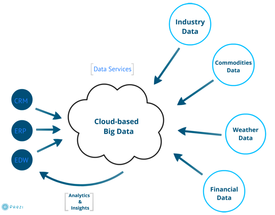
Project FAQ

Do I have to read every Slack post?

Yes.

There are relatively few posts in Slack, typically much less than 10 per week. If you were taking a live class I am sure you get also 10+ tips and comments from the instructors. Slack is a mechanism for us to communicate to the entire online class.

Use SLack to discuss things. You can also use it to discuss issues in your projects with other class mates openly.

I see something mssing or wrong in this FAQ. How can I correct or add it?

If you see something missing that we shoudl add, please edit this web page and create a pull request with your changes:

Edit here

Where to get help?

Please use Slack.

Do I have to work weekly on the project?

Yes.

Please plan to set aside a significant time every week for your project. We include your weekly progress in the grade. This is because you will fail if you do not set sufficient time aside and start your project in the week before the deadline.

When are updates due?

Updates are due every week from the time that the project has been announced. The updates will be committed by you to github.com. TAs will be reviewing your updates The weekly progress will be check by the TA’s while looking at the GitHub insights page.

TAs or instructors may make comments to your repository. It is your responsibility to make sure to stay in sync with the content in the repo. Best is to use a tool such as a command line tool or a GUI tool to stay in sync with the repo.

How do I define a project?

Please take a look at the class content and select a topic that interests you. Your project needs to be related to big data and provide an analysis of the data. You may choose a topic that is only explained later on in class. In this case, you can explore the topic ahead of time before it is explained in class. Previous class material is posted for all topics. If you have a question, work with the TA’s and instructors.

Please remember this is not just an AI class to demonstrate a specific AI method. Your project must have a section or an explanation of how your project relates or could relate to big data.

However, it is not required to use a huge dataset for this class.

The class has also the ability to do projects related to cloud infrastructure. In that case, please contact Gregor directly to assess if you have enough qualifications and can succeed in the project.

Project Directory

The following is the best structure for your project

project/project.md # your project report. This is a must.
project/project.bib # your project bib file if you use jabref
project/plan.md # for final submission move your Plan section here
project/images # place all images in this directory
project/code/

Move your python code or notebooks here.
project/data

Your project must not have (large) data in GitHub, instead you must have a program that downloads the data. best is to add project/data to your .gitignore file See more information on the data section.

Make sure you create in your paper citations and references to your own code and GitHub directory.

Filenames

Filenames must be precise, and we recommend using lower case file names in most cases (some Python class files may also contain capital letters). Filenames must not have spaces included in them. We will not review any information included in a file that contains spaces or characters that are not in [a-Z0-9] and the _ and - characters. We will return your project without review and assign an “F” as those files cause issues.

All image file names must be lower case.

Her an example of an image file name that is wrong in many ways:

project/images/THIS IS Gregor's Image.PNG

Images in reports must use the download link that is used in github as the link that you use to refer to it. If you see the word “blog” in it you have the wrong link. Take a look at our project example and carefully compare.

Wrong because

contains spaces contains
capital letters
contains ' which is not allowed ever
has an ending with capital letters

Project Proposal

This is a snapshot of your final project. You do not have to use the words I or plan simply write it as if you already decided to do the project and make it look like a final paper’s snapshot. Your paper must follow a typical research paper outline. The project ideally provides a novel feature that has not been presented by others. Just replication what others in the community did may not be lead to the best result. If you have not researched if others have done your project, It also will not lead to your best result.

A sample of a report is provided at

Sections that must be included

Abstract
Introduction
Related Research Identify similar projects and describe what you do differently
Data Write about which data you choose
Analysis Write about your intended analysis
Plan Provide a plan that lists what you do every week.(This plan is to be removed before the final submission at the end of the semester. You can move it into a file called project/plan.md in case you like to preserve it
Refernces

Please make sure that the refernce section is the last section in the document.

Reports without programming

It is possible for undergraduates, but not for graduate students to do a report that does not include programming. You will automatically get a half grade point deduction, and the best grade achievable will be an A-. The report will typically be 25% to 50% longer than a project with programming. It must be comprehensive and have a more in-depth background section. Proper citations are a must. Citations are typically much more in reports due to the nature of it.

In case you chose a report, your directory structure will look like this

report/report.md # your project report. This is a must.
report/report.bib # your project bib file
report/plan.md # for final submission move your Plan section here
report/images # place all images in thsi directory

It is our strong recommendation that you use jabref for assisting you with the management of your references! You will save a lot of time while using it and assure that the format will be correct, which is important for reports!

Formal writing

They shall not use the word “I” in the report.

We do allow, however, the words we, you, or the author

In general:

Do not use first-person pronouns (“I”, “me”, “my”, “us”, etc.). …
You must not use contractions such as don’t or ’ve …
Avoid colloquialism and slang expressions. …
Avoid nonstandard diction. …
When using an abbreviation, it must be defined before its first use in brackets): Artificial Intelligence (AI) … Avoid the creation of unnecessary abbreviations. It is better to say big data instead of BD
Avoid the overuse of short and simple sentences.
Avoid the overuse of very long and complex sentences.

colons

A colon is :

They shall not use a space before a colon ever.
They shall not use colons in section headers.

Quotes

They shall not use “quoted quotes” to highlight.
They shall use italic to highlight

Quotes are reserved for citations and must be followed by a citation that is included in your reference section.

Update and check the submission

Once you submit your paper, you need to dow the following.

modify the README.yaml file and update the information of your project in it. Keep it up to date in case authors or title changes. We use this information to mine all Gitrepos, and thus it must be up to date all the time. In case you are in a group, make sure you preserve the authors' order in the list among all group members. The person that has the repo for the project must be the first author.

Example for single author: https://github.com/cybertraining-dsc/fa20-523-312/README.yaml
Check every week if your report renders correctly and if your report is listed at https://cybertraining-dsc.github.io/report/ Click on your paper link, your student link, and your edit link to ensure they all work correctly. If not, please correct them via a pull request (you can edit that page and see how we do it for other students).

Using Markdown

We no longer accept any document format that is not markdown. We use proper markdown that must not include any HTML tags. submissions with HTML tags will be rejected without reviews. You must look at our template in raw format to see what features of markdown we use. Your file may not be properly rendered in GitHub (e.g., abstract and table of content, as well as references look differently), but it will be on our Web site.

References and citations

You must have a reference section from the get-go. We use footnotes to showcase the references as GitHub does not support proper references in markdown. However, we use footnotes in a straightforward and specific way that requires you to be careful with the dot at the end of the sentence. The footnotes must not be after the dot, but they must be within the dot. The reason is that at one point, we will automatically replace your footnotes with a [number] theme. You do not have to do this; we will do this. This is simpler than it sounds for you, so we give an example:

When you use the citations, you MUST for us do them before the dot that closes the sentence that you cite in or refers to. They do require you do the [^1] before the dot

wrong: This is a sentence with reference.[^1]

correct: This is a sentence with reference [^1].

wrong: Simon says "Hallo".[^1]

The reference section must be the last section in your report

## 8. Refernces

[^1]:  This is where you put the citation information.

See, there is no space before the :

Please make sure that different refernces are separated by an empty line.

As with any class, you need to know what plagiarism is and how to avoid it. If you need more information, check out our notes in the book “Scientific Writing with Markdown”. Make sure you know how to cite and use proper punctuation after the citation. E.g.

This is a wrong citation. [1]

[1] This is a wrong citation.

This is a correct citation [1].

Note the position of the . and the [1]

Also in most cases, we do not care who said what, while in Engilsh, business, or psychology you emphasize this leading often to complex sentences.

Example:

Once upon a time, there was a scientist called von Neuman that introduced a computing machine for weather predictions while being a researcher at Institute XYZ [1].

Instead, it is often better to just write:

Computers were used for weather prediction early on [1].

Please note that there is quite a difference between these citation styles. Shorter is often better.

Format of References

Although we use footnotes in markdown, we will use the propper IEEE format style for citations. Please google it. The easiest way for you to get IEEE references is to use jabref and manage your references there and just copy the rendered content from jabrefs display window into your markdown reference section. Make sure to remove all HTML tags. If you use jabref, please submit your references as project.bib file

URLs in the text

In case you use URLs in the text, they must be followed by a citation with it being referenced in the reference section by a label.

References that are not cited in the text

You must not have any references that you have not cited in the text

Images that you copied

In case you copied an image from the internet, it must have a citation in the caption and be referenced in the reference section.

If you use figures, check carefully with our template, do not invent your own method. We will reject your paper without review if you do it wrong.

How to include images

We have provided a clear example. Do not invent your own method or use relative links. Images must be cited with a link to the raw image in GitHub. See our example!

Programs

Python

You are allowed to use python notebooks or python programs. All of which must be checked into GitHub in your assigned repo. Sometimes notebooks have a cache that is too big for GitHub, this you need to make sure to always clear the cache before you check it into GitHub.

Otherprogramming langauges

Use python.

Data

Please add a “download” data function that downloads the data from the source. Do not store the actual data in Github. The download function must have a logic that does not download the data when it is already downloaded. Python makes this easy with os.path and python requests. We recommend you use python requests and not urllib. You can share the download function openly with each other.

Images from Programs

You can create png files of graphics so you can include them in your project.md. Make sure you add a save image function and do not just create screenshots. Matplotlib and other graphics frameworks have an API call for this.

There are many good and even specialized graphics libraries that you can use, examples are

matplotlib
bokeh
seaborn
…

If you copy the image from somewhere, you must create a citation in the caption. If you did this figure yourself, you do not have to do that. See Plagiarism rules.

Bechmark

Your program must use cloudmesh benchmark. It includes a convenient StopWatch and benchmark print function.

see: https://colab.research.google.com/drive/1tG7IcP-XMQiNVxU05yazKQYciQ9GpMat#scrollTo=TZAjATZiQh4q&uniqifier=1

Template Links

Here are the relevant URLs to them, which you naturally can find from our report web page. But as some of you have not visited the web page at

See that githib does not quite render it properly, but it will by ok for a superficial view and editing.

https://github.com/cybertraining-dsc/fa20-523-312/blob/main/project/project.md

Make sure to check your report at

https://cybertraining-dsc.github.io/report/

which will be updated weekly

5 - Tutorials

New: Experimental feature to publish tutorials that have been presented in various classes and provide general usefulness. Howver our PDF books include much more detailed information.

5.1 - cms

Selected Tutorials for cloudmesh shell

5.1.1 - Using Shell.download to Download Files

Using Shell to download files that can be potentially very large in python.

Learning Objectives

Install cloudmesh.common
Use Shell.download from cloudmesh-common to download files from the internet.

Requirements

python3 --version > 3.8

Topics covered

Python 3 `venv`

Best practice is to use a venv in python to isolate your custom python instalation:

$ python3 -m venv ~/ENV3
$ source ~/ENV3/bin/activate

$ ~/ENV3/Scripts/activate.exe

in Windows gitbash.

Installation of `cloudmesh.commn`

Install cloudmesh-common with:

pip install -U pip
pip install cloudmesh-common

Usage of `Shell.download`

Shell.download leverages the streaming capabilities of the requests library for large files.

Example download of image where underlying downloader is requests:

$ python3
Python 3.9.4 (v3.9.4:1f2e3088f3, Apr  4 2021, 12:32:44)
[Clang 6.0 (clang-600.0.57)] on darwin
Type "help", "copyright", "credits" or "license" for more information.

>>> from cloudmesh.common.Shell import Shell
>>> file_url = 'https://github.com/cloudmesh/pi/blob/main/content/en/tutorial/example/featured-image.png?raw=true'
>>> destination = '~/Desktop/image.png'
>>> Shell.download(file_url, destination)
/users/you/Desktop/image.png: 100%|#########| 22.6k/22.6k [00:00<00:00, 3.58MB/s]
'/users/you/Desktop/image.png'

Configuring the Download Cache

Shell.download only downloads if the filename in the destination does not already exist. If you like to change the behavior and ignore it, you need to use the force parameter.

Shell.download(file_url, destination, force=True)

Different Providers for `Shell.download`

Example where provider is system. Cloudmesh Shell will first try to use wget then curl (if wget fails)

$ python3
Python 3.9.4 (v3.9.4:1f2e3088f3, Apr  4 2021, 12:32:44)
[Clang 6.0 (clang-600.0.57)] on darwin
Type "help", "copyright", "credits" or "license" for more information.

>>> from cloudmesh.common.Shell import Shell
>>> file_url = 'https://github.com/cloudmesh/pi/blob/main/content/en/tutorial/example/featured-image.png?raw=true'
>>> destination = '~/Desktop/image.png'
>>> Shell.download(file_url, destination, provider='system')
sh: wget: command not found
  % Total    % Received % Xferd  Average Speed   Time    Time     Time  Current
                                 Dload  Upload   Total   Spent    Left  Speed
100   153  100   153    0     0    467      0 --:--:-- --:--:-- --:--:--   467
100   164  100   164    0     0    379      0 --:--:-- --:--:-- --:--:--   379
100 22590  100 22590    0     0  43694      0 --:--:-- --:--:-- --:--:-- 43694
INFO: Used curl
'/users/you/Desktop/image.png'
>>>

We can see here that Shell.download uses curl and not wget. This is because the example system did not have wget as a terminal ('system') command installed.

Installing other Download Programs

Your OS typically has defined mechanisms to install commands such as curl and wget. If they are not installed. Shell.download will use Python requests automatically. If you like to use wget r curl you need to install them.

On Ubuntu you can fro example say

$ sudo apt install wget

$ sudo apt install curl

Please find the method that works for your system, or use the default method which does not require a third party provider.

The order of the providers is defined as

wget
curl
Python requests

We use wget and curl first as many OS have optimized versions of them.

5.2 - Git

Selected tutorials that make the use of GitHub easy.

5.2.1 - Git pull requst

We provide a practical guide on how to do GitHub pull requests from the commandline and the GUI for this Web site.

It is very easy to help us modifying the Web Site through GitHub pull requests. We demonstrate this via the commandline and via the GitHub GUI.

The commandline can be run form any computer with Linux, Windows, and macOS. ON Windows you need to install gitbash and use that. THis way you have a commandline terminal that just works like on LInux and OSX.

Github Pull Request via the commandline

9:15 min

Github Pull Request via the GitHub GUI

5.2.2 - Adding a SSH Key for GitHub Repository

Scary SSH Keys are Now a Breeze

Jacques Fleischer, Gregor von Laszewski

Abstract

We present how to configure an SSH Key on GitHub so that you can clone, commit, pull, and push to repositories. SSH keys provide an easy way to authenticate to github. Together with ssh-agent and ssh-add it allows you to do multiple commtits without having to retype the password.

Contents

Keywords: ssh

Documentation for Linux and macOS

Please follow the Windows documentation, but instaed of using gitbash, pleas use the regular terminal. on macOS, make sure you have xcode installed.

Uploading the SSH key

Please ensure that you have Git (Git Bash) and a repository on GitHub. This tutorial assumes you already have a GitHub repository as well as a GitHub account.

Open Git Bash by pressing the Windows key, typing git bash, and pressing Enter.
Then, go on GitHub, click on your profile icon in the top right, click Settings, and click SSH and GPG keys on the left hand side. Confirm that there are no SSH keys associated with your account. If there are keys, then perhaps you have made some already. This tutorial focuses on creating a new one.
Go back to Git Bash and type ssh-keygen. Press Enter. Press Enter again when it asks you the file in which to save the key (it should say Enter file in which to save the key (/c/Users/USERNAME/.ssh/id_rsa):.
1. If you have already created a key here, it will ask you if you would like to overwrite the file. Type y and press Enter.
Enter a password that you will remember for your SSH key. It will not appear as you type it, so make sure you get it right the first time. Press Enter after typing the password that you come up with.
After seeing the randomart image associated with your SSH, you should be able to type a new command. Type cat ~/.ssh/id_rsa.pub and press Enter. Your key will appear— remember that this should not be shared with others. The key begins with ssh-rsa and it may end with your username. Copy this entire key by clicking and dragging over it, right-clicking, and clicking Copy.
Return to your web browser which is on the GitHub SSH key settings page. Click the green button that reads New SSH Key and type a Title for this key. You should name it something memorable and distinct; for example, if you just generated the key on your desktop computer, a suitable name is Desktop. If generated on your laptop, name it Laptop, or if you have numerous laptops, differentiate them with distinct names, and so on.
1. If you only have one computer and you have preexisting keys on this page, maybe some which you do not remember the password to or have fallen out of use, consider deleting them (as long as you are sure this will not break anything).
Paste the key into the key box. You should have copied it from Git Bash in Step #5. Then, click the green button that reads Add SSH key. Congratulations— you have successfully configured your SSH key.

Using the ssh key

Now we will try cloning a repository. We use as an example a repository that we created for a student from a REU. Your example may be different. please adjust the repository name. Your repository will have a format of xxxx-reu-xxx

Navigate to your repository and cd into it. (In case of the REU we recommend to place it into a directory called cybertraining-dsc.
```
$ mkdir ~/Descktop/cybertraining-dsc 
$ cd cybertraining-dsc
$ git clone git@github.com:cybertraining-dsc/YOURREPONAME.git
```
and replace YOURREPONAME with the name of your repository
Alternatively you can download it via the GitHub Web GUI. Once you are on your repository page, click the green button that reads Code with a download symbol. Click the SSH option and click on the clipboard next to the link so that you copy it. It should say Copied! after you click on it.
Decide where you want your repository folder to be stored. This tutorial will clone the repo into the Documents folder. Go back to Git Bash and type cd ~/Desktop/cybertraining-dsc and press Enter. It is a good idea to create a folder titled reu for organization. Type mkdir reu and press Enter. Type cd reu and press Enter. Finally, type git clone, and after you put a space after clone, paste the copied link from GitHub. For example, your command should look similar to this: git clone git@github.com:cybertraining-dsc/su21-reu-361.git Then, press Enter.
1. The shortcut Ctrl + V does not work in Git Bash for pasting. Instead, you can press Shift + Insert to paste.
Type in your password for your SSH key and press Enter. The repo should clone with no issue. You can now type code . and press Enter to open VSCode in this directory. Click Yes, I trust the authors if prompted in VSCode. If you use PyCharm instead of VSCode, you can open it from Windows search; inside of PyCharm, click File, Open... and then navigate to C:, Users, your username, Documents, and then click on reu so it is highlighted in blue and then click OK. If PyCharm asks, you can choose to open it in This Window or a New Window.

Using ssh-agent and ssh-add

If you do not want to always type in your password you can prior to the first commit in the termnal in which you issue the commits say

$ eval `ssh-agent`
$ ssh-add

5.2.3 - GitHub gh Command Line Interface

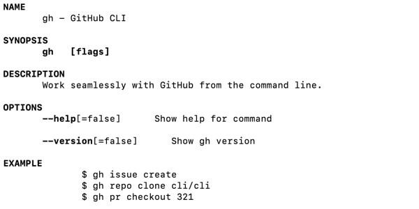
A brief tutorial on the installation and usage of the GitHub gh CLI

Figure 1: GitHub Command gh.

GitHub provides an extended gh commandline tool that allow easy interaction of forking repositories directly from github. IT also provides additional fimctionality to interact with other advanced features that are typically not provided in the git command tool.

Learning Objectives

Learn how to install the gh command
Learn how to use the gh command

Topics covered

1. Introduction

The new GitHub gh command allows GitHub users to work from the terminal of their machine without having to visit the web browser GUI to manage things like issues, PRs, and forking. We will show you what features it provides and how to use it. The gh command provides useful features that is not provided by the `git commandline tool.

2. Installing GitHub gh command

Visit the GitHub CLI homepage at https://cli.github.com/ for installation instructions. We recommend that you check out the source distribution because We found that whne we did this tutorial not all features were included in the brew instalation. We assume ths will cahnge over time and you may soon be able to just use the bre install on LInux and MacOs.

On mac, you can use the following command with Brew:

brew install gh

For Windows useser, please follow the install instructions fro Winodws.

3. Logging in with GitHub gh Command

It is best practice to be using SSH-keys with GitHub. Create one if you have not already with the following command:

ssh-keygen

We recommend t use the the default location.

To authenticate with the GitHub gh comamand, run the following command. We have included the answers to the interactive prompts used for this guide.

gh auth login

What account do you want to log into? GitHub.com
? What account do you want to log into? GitHub.com
? What is your preferred protocol for Git operations? SSH
? Upload your SSH public key to your GitHub account? ~/.ssh/id_rsa.pub
? How would you like to authenticate GitHub CLI? Login with a web browser

! First copy your one-time code: 1234-1A11
- Press Enter to open github.com in your browser...

3.1 Adding Additional Keys

IN acse you work with multiple computers it is advisable to add your keys from these machines also. We demonstarte the interaction to upload the key from a new machine.

newmachine$ gh ssh-key add ~/.ssh/id_rsa.pub 
Error: insufficient OAuth scopes to list SSH keys
Run the following to grant scopes: gh auth refresh -s write:public_key
newmachine$ gh auth refresh -s write:public_key

! First copy your one-time code: 4C2D-E896
- Press Enter to open github.com in your browser... 
✓ Authentication complete. Press Enter to continue...

newmachine$ gh ssh-key add ~/.ssh/id_rsa.pub   
✓ Public key added to your account

4. Forking

We can easily create a fork of a repo with the following:

gh repo fork

This is useful for when you do not have write access to the original repository.

5. Pull Requests

We can create a pull request easily as follows from a git repo:

gh pr create

The command above will ask the user where to push the branch (if it does not already exist on the remote). It will also offer the option to fork the initial repository. You will want to do this if you do not have write access to the original repo.

Once created, you may view the status of the PR with the following:

gh pr status

Reviewers can checkout your pull request to verify changes as follows:

gh pr checkout {PR NUMBER}

The reviewer can then approve the PR as follows:

gh pr review --approve

Subsequently, the PR can be merged as follows:

gh pr merge {PR NUMBER}

You may also list all pull requests with the following:

gh pr list

Finally, PRs can be closed with

gh pr close {PR NUMBER}

6. Managing Issues with GitHub gh Command

To create an issue, call the following:

gh issue create --title="Bug 1" --body="description"

We can also check the status of issues relevant to use with:

gh issue status

Alternatively, we may list all open issues.

gh issue list

Finally, we may close issues with:

gh issue close {ISSUE NUMBER}

7. Manual Pages

7.1 gh

gh(1)                                                                    gh(1)

NAME
       gh - GitHub CLI

SYNOPSIS
       gh   [flags]

DESCRIPTION
       Work seamlessly with GitHub from the command line.

OPTIONS
       --help[=false]      Show help for command

       --version[=false]      Show gh version

EXAMPLE
              $ gh issue create
              $ gh repo clone cli/cli
              $ gh pr checkout 321

SEE ALSO
       gh-alias(1),  gh-api(1),  gh-auth(1),  gh-completion(1),  gh-config(1),
       gh-gist(1),   gh-issue(1),   gh-pr(1),    gh-release(1),    gh-repo(1),
       gh-secret(1), gh-ssh-key(1)

7.2 List of Man Pages

Tha manual pages are published at the gh manual. For mor information you can also use the man command. A full list of manual pages includes:

gh
gh-alias-delete
gh-alias-list
gh-alias-set
gh-alias
gh-api
gh-auth-login
gh-auth-logout
gh-auth-refresh
gh-auth-status
gh-auth
gh-completion
gh-config-get
gh-config-set
gh-config
gh-gist-clone
gh-gist-create
gh-gist-delete
gh-gist-edit
gh-gist-list
gh-gist-view
gh-gist
gh-issue-close
gh-issue-comment
gh-issue-create
gh-issue-delete
gh-issue-edit
gh-issue-list
gh-issue-reopen
gh-issue-status
gh-issue-view
gh-issue
gh-pr-checkout
gh-pr-checks
gh-pr-close
gh-pr-comment
gh-pr-create
gh-pr-diff
gh-pr-edit
gh-pr-list
gh-pr-merge
gh-pr-ready
gh-pr-reopen
gh-pr-review
gh-pr-status
gh-pr-view
gh-pr
gh-release-create
gh-release-delete
gh-release-download
gh-release-list
gh-release-upload
gh-release-view
gh-release
gh-repo-clone
gh-repo-create
gh-repo-fork
gh-repo-view
gh-repo
gh-secret-list
gh-secret-remove
gh-secret-set
gh-secret
gh-ssh-key-add
gh-ssh-key-list
gh-ssh-key

7. Conclusion

There are many other commands for the GitHub CLI that can be found in the gh manual, however we only include a select number of relevant commands for this guide. The commands mentioned above serve to familiarize the user with the GitHub CLI while also providing practical usage.

5.2.4 - GitHub hid Repository

Using the student hid directory

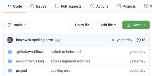
Figure 1: GitHub hid directory.

To contribute to our open source projects we provide you with a Git repository in which you conduct your activities.

https://github.com/cybertraining-dsc

Learning Objectives

Learn how to cone the repo
Learn how to use the rego
Learn how to commit and push changes to GitHub

Topics covered

1. Introduction

As part of our open source activities, you will be given a GitHub repository. To contribute to our open source projects we provide you with a Git repository in which you conduct your activities.

https://github.com/cybertraining-dsc

We will explain how you use them from the command line.

2. Prerequisites

On macOS we assume you have x-code installed which comes with the git command
line tools On Windows we assume you have gitbash installed and use git
through gitbash. Alternatively, you can use multipass, or WSL2 On Linux, make
sure you have the git command line tools installed.

3. Setting up the ssh-key

In case you have not yet set up an ssh key, you can do this with the command.

$ ssh-keygen

YOu will be asked for the default location, accept it. After that, you will be asked for a passphrase. Please choose one and make sure you do not make it empty. Often you find wrong tutorials or guidance by others that say you can leave it empty. DO NOT FOLLOW THEIR WRONG ADVICE.

Upload the content of the file

$ cat ~/.ssh/id_rsa.pub

Into the GitHub portal at https://github.com/settings/keys. You will then use the SSH key to authenticate to GitHub. To not always have to type in the password you can use ssh-keychain. On Mac OS you can simply use the command

$ ssh-add

and enter your password

4. Simplify the Tutorial while using Shell Variables

To simplify the tutorial we use from here on two shell variables. The first is HID which specifies the name of your GitHub repository as found in

https://github.com/cybertraining-dsc

In our case, we use hid-example. The second variable is the name/path of the editor in which we edit commit messages for git.

$ export HID=hid-example
$ export EDITOR=emacs

5. Cloning the Repository

Let us now clone the repository, change int the checked out repository and edit the project file.

$ git clone git@github.com:cybertraining-dsc/$HID.git
$ cd $HID/project
$ $EDITOR index.md

Now let us make a modification and save the file locally.

6. Commit Changes Locally

To commit the changes locally, you use the following command. Make sure to put a commit message and specify the filename.

$ git commit -m "Improved document with this and that" index.md

7. Adding Files

To add new files you can simply use the add command and use the commit command after it.

$ git add image/newimage.png
$ git commit -m "Improved document with this and that" image/newimage.png

8. Push the commits to GitHub

GitHub as you know is a service that stores your files once you push them from your local commits to GitHub. To push the commits use the command

$ git push

8. Pulling Changes

GitHub shines when you work with multiple people together on your projects. This may be project partners or feedbacks that are placed in your documents by us. Thus, it is important that you state in synchronization with the files in GitHub. Do this use the command

$ git pull

in any directory of the repository that you have checked out. It will update any file that has changed. In case of a conflict, your file will include a text such as

<<<<<<< HEAD
This is the new text from you
=======
This is the text in the repo
>>>>>>>

You will have to remove the text between the «< and »> and replace it with the text that is correct. In the simplest case, one of the choices will be correct. However, you may have in some cases to merge the two versions.

It is important to pull frequently. It is also important to not just paste and copy the entire file, but use the command line tools and editor to conduct the change as not to overwrite other changes.

7. Conclusion

The use of git from the command line is straightforward for existing repositories. It is easy to do. Make sure to create an ssh-key and start in synchronization with frequent pulls.

5.3 - REU Tutorials

New: A number of smaller tutorials useful for the REU 2021.

5.3.1 - Installing PyCharm Professional for Free

This tutorial teaches how to get PyCharm Professional for free on Windows 10 using a university email address.

Abstract

This tutorial teaches how to get PyCharm Professional for free on Windows 10 using a university email address. You can follow a similar process on Linux and macOS.

Contents

Keywords: pycharm

Steps

Click the following image to be redirected to a YouTube video tutorial for installing PyCharm Professional.

Please ensure that you qualify. This includes you having a valid educational email or be part of an open-source project. Make sure to explore the license agreements for PyCharm as they may change.

Open up a web browser and search pycharm. Look under the link from jetbrains.com and click Download PyCharm.
Click the blue button that reads Download under Professional. Wait for the download to complete.
Open the completely downloaded file and click Yes on the UAC prompt.
1. If you have a school computer, please refer to the note under step 5 of the Windows section in the Python tutorial found here: https://github.com/cybertraining-dsc/cybertraining-dsc.github.io/blob/main/content/en/docs/tutorial/reu/python/index.md
Click Next, click Next again, and check the box that reads Add launchers dir to the PATH. You can also create a Desktop Shortcut and create the .py association if you would like. The association changes which program, by default, opens .py files on your computer.
Click Next and then click Install. Wait for the green progress bar to complete. Then, you must restart your computer after making sure all of your programs are saved and closed.
Open PyCharm either by clicking on the Desktop shortcut you might have made or hit the Windows key and type PyCharm and choose the program from the search results.
Check the box that says I confirm that I have read and accept the terms... after agreeing to the terms.
Click Continue. You can choose to send anonymous statistics, if you want to; click the option you want.
Click the hyperlink that says Buy license in the top right of the window. Do not worry — you will not be spending a cent.
Click the person icon in the top right of the page (if you cannot find this person icon, then click this link and hopefully, it still works: https://account.jetbrains.com/login ).
Create a JetBrains account by entering your university email address. Click Sign Up after entering your email; then, you have to go on your email and confirm your account in the automated email sent to you. Click Confirm your account in the email.
Complete the registration form and click Submit.
Click Apply for a free student or teacher license. Scroll down and click the blue button that reads Apply now.
Fill out the form using your (educational) email address and real name. Check the boxes if they apply to you. Then click APPLY FOR FREE PRODUCTS.
JetBrains should send you an automated email, ideally informing you that your information has been confirmed and you have been granted a free license. If it does not arrive immediately, wait a few minutes. Go back to PyCharm and sign in with your JetBrains account after receiving this email. Click Activate. Now you can use PyCharm.

5.3.2 - Installing Git Bash on Windows 10

Installung Git.

Abstract

This tutorial teaches how to install Git and Git Bash.

Contents

Keywords: git

Windows

Click the following image to be redirected to a YouTube video tutorial for installing Git and Git Bash. This same video also includes instructions to create a virtual Python environment, which you can do as well.

To verify whether you have Git, you can press Win + R on your desktop, type cmd, and press Enter. Then type git clone and press Enter. If you do not have Git installed, it will say 'git' is not recognized as an internal or external command...

As long as Git does not change up their website and hyperlinks, you should be able to download Git from here and skip to step 2: https://git-scm.com/downloads

Open a web browser and search git. Look for the result that is from git-scm.com and click Downloads.
Click Download for Windows. The download will commence. Please open the file once it is finished downloading.
The UAC Prompt will appear. Click Yes because Git is a safe program. It will show you Git’s license: a GNU General Public License. Click Next.
1. The GNU General Public License means that the program is open-source (free of charge).
Click Next to confirm that C:\Program Files\Git is the directory where you want Git to be installed.
Click Next unless you would like an icon for Git on the desktop (in which case you can check the box and then click Next).
You will be asked several questions for the setup. We recommend the following settings:
- Click Next to accept the text editor,
- Click Next again to Let Git decide the default branch name
- Click Next again to run Git from the command line and 3rd party software,
- Click Next again to use the OpenSSL library
- Click Next again to checkout Windows-style,
- Click Next again to use MinTTY,
- Click Next again to use the default git pull,
- Click Next again to use the Git Credential Manager Core,
- Click Next again to enable file system caching, and then
- Click Install because we do not need experimental features.
The progress bar should not take too long to finish. To test if it is installed, you can search for Git Bash in the Windows search now to run it.

5.3.3 - Using Raw Images in GitHub and Hugo in Compatible Fashion

We need raw images

This tutorial teaches how to add images on GitHub and use them in your markdown file that can be rendered in Hugo and markdownon GitHub.

Contents

Keywords: github

Steps

Upload your image to GitHub in the images directory
Click on the image file and then right click on it and click Open image in new tab
Use the URL shown in the address bar of the new tab to paste into the markdown file.
When using the file, please add a caption; also, if it is copied, make the citation which should point to the reference section

![database sample](https://github.com/cybertraining-dsc/cybertraining-dsc.github.io/raw/main/content/en/docs/tutorial/reu/github/images/images-download.png)

**Figure 2:** Sample Database file obtained from the USGS
water-quality database for the year 2017 [^1]

## Refernces

[^1]: HERE COMES THE CITATION OF THE IMAGE

5.3.4 - Using Raw Images in GitHub and Hugo in Compatible Fashion

We need raw images

This tutorial teaches how to add images on GitHub and use them in your markdown file that can be rendered in Hugo and markdownon GitHub.

Contents

Keywords: github

How to use images is clearly shown in our template at

https://github.com/cybertraining-dsc/hid-example/blob/main/project/index.md

5.3.5 - Uploading Files to Google Colab

Google Drive File upload for Google Colab

Abstract

This tutorial teaches how to import CSV’s into a Google Colab .ipynb.

Contents

Keywords: colab

Note

There are two different methods of uploading files to Google Colab Jupyter notebooks. One way is to have the user upload the file to the user’s Google Drive before running the notebook. Another way is to have the notebook ask the user to upload a file directly into the notebook from the user’s computer. This tutorial outlines both ways.

The notebook code with both methods can be found here

Read File from Drive

This code will read a CSV file using pandas. Before running it, the user must upload the CSV file to the Google Drive of the same Google account on which it runs the notebook in Colab (e.g., your account). The CSV file in this example is titled kag_risk_factors_cervical_cancer but please rename it accordingly to match the file you would like to upload.

Cell 1:

import pandas as pd
from google.colab import drive 
drive.mount("/content/gdrive", force_remount=True)
# The next line of code will tell Colab to read kag_risk_factors_cervical_cancer.csv in your Drive (not in any subfolders)
# so you should alter the code to match whichever .csv you would like to upload.
df=pd.read_csv('gdrive/My Drive/kag_risk_factors_cervical_cancer.csv')
# The next two lines of code convert question marks to NaN and converts values to numeric type, consider 
# removing the next two lines if not necessary.
df = df.replace('?', np.nan) 
df=df.apply(pd.to_numeric)
# If this cell successfully runs then it should output the first five rows, as requested in the next line of code
df.head(5)

Colab will ask you to click on a blue link and sign in with your account. Once done, the user must copy a code and paste it into the box on Colab for authentication purposes. Press Enter after pasting it into the box.

If it outputs an error along the lines of unknown directory, try rerunning the two cells and ensuring that your CSV is not in any folders inside Google drive. You can also alter the code to point it to a subdirectory if needed.

Read File from Direct Upload

To read it with built-in Colab methods, you can use the following code:

Cell 1:

from google.colab import files
df = files.upload()

The user will be prompted to click Browse... and to find the file on the user’s local computer to upload. Sometimes trying to upload the file will give this error:

MessageError: RangeError: Maximum call stack size exceeded.

In this case, the user should click the folder icon on the left side of Google Colab window, then the paper with an arrow icon (to upload a file), then upload the CSV you wish to use. Then rerunning Cell 1 is not necessary. Simply proceed to Cell 2. If this still does not work, see this stackoverflow page for further information.

Cell 2:

df=pd.read_csv('kag_risk_factors_cervical_cancer.csv')
# The next two lines of code convert question marks to NaN and converts values to numeric type, consider 
# removing the next two lines if not necessary.
df = df.replace('?', np.nan) 
df=df.apply(pd.to_numeric)
# If this cell successfully runs then it should output the first five rows, as requested in the next line of code
df.head(5)

Remember to rename the instances of kag_risk_factors_cervical_cancer.csv accordingly so that it matches your file name.

Acknowledgments

Credit to Carlos who provided the cell to upload the file directly.

5.3.6 - Adding SSH Keys for a GitHub Repository

Using SSH keys with GitHub

This tutorial teaches how to configure an SSH Key on GitHub so that you can clone, commit, pull, and push to repositories (repos).

Contents

Keywords: ssh

Windows

Please ensure that you have Git (Git Bash) and a repository on GitHub. This tutorial was created with the REU program in mind, where the students are provided with a GitHub repository. If you are not in REU, then you can create a new repository on GitHub and clone that instead.

Open Git Bash by pressing the Windows key, typing git bash, and pressing Enter.
Then, go on GitHub, click on your profile icon in the top right, click Settings, and click SSH and GPG keys on the left hand side. Confirm that there are no SSH keys associated with your account. If there are keys, then perhaps you have made some already. This tutorial focuses on creating a new one.
Go back to Git Bash and type ssh-keygen. Press Enter. Press Enter again when it asks you the file in which to save the key (it should say Enter file in which to save the key (/c/Users/USERNAME/.ssh/id_rsa):.
1. If you have already created a key here, it will ask you if you would like to overwrite the file. Type y and press Enter.
Enter a password that you will remember for your SSH key. It will not appear as you type it, so make sure you get it right the first time. Press Enter after typing the password that you come up with.
After seeing the randomart image associated with your SSH, you should be able to type a new command. Type cat ~/.ssh/id_rsa.pub and press Enter. Your key will appear— remember that this should not be shared with others. The key begins with ssh-rsa and it may end with your username. Copy this entire key by clicking and dragging over it, right-clicking, and clicking Copy.
Return to your web browser which is on the GitHub SSH key settings page. Click the green button that reads New SSH Key and type a Title for this key. You should name it something memorable and distinct; for example, if you just generated the key on your desktop computer, a suitable name is Desktop. If generated on your laptop, name it Laptop, or if you have numerous laptops, differentiate them with distinct names, and so on.
1. If you only have one computer and you have preexisting keys on this page, maybe some which you do not remember the password to or have fallen out of use, consider deleting them (as long as you are sure this will not break anything).
Paste the key into the key box. You should have copied it from Git Bash in Step #5. Then, click the green button that reads Add SSH key. Congratulations— you have successfully configured your SSH key. Now we will try cloning your REU repository.
Navigate to your repository. It should be in the cybertraining-dsc directory with a name format of xxxx-reu-xxx. Once you are on that page, click the green button that reads Code with a download symbol. Click the SSH option and click on the clipboard next to the link so that you copy it. It should say Copied! after you click on it.
Decide where you want your repository folder to be stored. This tutorial will clone the repo into the Documents folder. Go back to Git Bash and type cd ~/Documents and press Enter. It is a good idea to create a folder titled reu for organization. Type mkdir reu and press Enter. Type cd reu and press Enter. Finally, type git clone, and after you put a space after clone, paste the copied link from GitHub. For example, your command should look similar to this: git clone git@github.com:cybertraining-dsc/su21-reu-361.git Then, press Enter.
1. The shortcut Ctrl + V does not work in Git Bash for pasting. Instead, you can press Shift + Insert to paste.
Type in your password for your SSH key and press Enter. The repo should clone with no issue. You can now type code . and press Enter to open VSCode in this directory. Click Yes, I trust the authors if prompted in VSCode. If you use PyCharm instead of VSCode, you can open it from Windows search; inside of PyCharm, click File, Open... and then navigate to C:, Users, your username, Documents, and then click on reu so it is highlighted in blue and then click OK. If PyCharm asks, you can choose to open it in This Window or a New Window.

5.3.7 - Installing Python

Installing Python

Abstract

This tutorial teaches how to install Python on Windows 10. It can be similarly installed also on macOS and Linux.

Contents

Keywords: python

Windows

Click the following image to be redirected to a 2-minute YouTube walkthrough.

First, open the url https://www.python.org/downloads/ in any web browser.
As of June 2021, the latest version of Python is 3.9.6. You may see a different number. We recommend you use the newest official version which is provided to you by simply clicking the button under “Download the latest version for Windows”.
Once the download has completed, open the file by clicking on it in your Downloads pane.
Be sure to check the box that reads “Add Python x.x to PATH”. This will allow you to run commands from the terminal/command prompt.
Click “Install Now”. The default options that entail this selection are appropriate.
1. The UAC prompt will pop up. UAC stands for “User Account Control” and exists so that the computer will not have unauthorized changes performed on it. Click “Yes” because Python is safe. School-issued computers may ask for an administrator password, so contact your IT department or professor.
The installation will take some time.
If the setup was successful, then it will say so. Click “Close”.
Click the “Type here to search” box in the bottom-left of the screen, type “cmd”, and press Enter.
1. An alternative method is to press the Windows key and the “R” key at the same time, type “cmd”, and press Enter. This is convenient for those who like to use the keyboard.
Type python --version and the output should read “Python x.x.x”; as long as it is the latest version from the website, congratulations. Python is installed on the computer.

Mac

Click the following image to be redirected to a 5-minute YouTube walkthrough. (Yes, Mac’s video is a little longer, but do not fret! You can skip to the 1:00 minute mark if you are in a hurry.)

First, open the url https://www.python.org/downloads/ in any web browser.
Underneath Download the latest version for Mac OS X, there should be a yellow button that reads Download Python x.x.x. Click on it, and the download should commence.
Once the download finishes, open it by clicking on it. The installer will open. Click Continue, click Continue again, and click Continue again. Read the agreements.
Click Agree.
1. If you want to check how much free storage you have on your computer, click the Apple icon in the top left of your computer. Click About This Mac and then click on Storage. As of July 2021, Python takes ~120 MB of space. Remember that 1 GB = 1000 MB.
Click Install. Enter your password and press Enter. The installation will take a while.
A Finder window will open. You can close it as it is unnecessary. Click Close in the bottom-right of the installer. Click Move to Trash because you do not need the installer anymore.
Next confirm that Python installed correctly. Click the magnifying glass in the top-right of your screen and then type terminal into Spotlight Search. Double-click Terminal.
1. The terminal will be used frequently. Consider keeping it in the dock for convenience. Click and hold the Terminal in the dock, go to Options, and click Keep in Dock.
Type python3 --version into the terminal and press Enter. It should output the latest version of Python. Congratulations!

Linux

Click the following image to be redirected to a 9-minute YouTube walkthrough. (Linux’s tutorial is the longest, but it is worth it.) This tutorial uses Ubuntu, but it should work on other Linux distros, as well.

Naturally we recommend that you read all of the licensing information.

First, open the url https://www.python.org/downloads/ in any web browser.
Look at the latest version. It is on the yellow button: Download Python x.x.x. You do not need to click this button. Remember this version number.
Open a terminal by pressing the Windows key or by clicking the grid on the bottom left of your screen. Type terminal. Click on the Terminal result that appears.
Next, prepare your system:

Note: If you want to check how much disk space you have, you can use

$ df -h /
Filesystem       Size   Used  Avail Capacity iused       ifree %iused  Mounted on
/dev/disk1s5s1  1.8Ti   14Gi  387Gi     4%  553757 19538475003    0%   /

The value under Avail will be your available space. Make sure you have sufficient space.

$ sudo apt-get update
$ sudo apt install -y wget curl
$ sudo apt install -y openssl libssl-dev
$ sudo apt install -y build-essential zlib1g-dev libncurses5-dev 
$ sudo apt install -y libgdbm-dev libnss3-dev  libreadline-dev libffi-dev libsqlite3-dev libbz2-dev

After this finishes, type cd /opt and press Enter. Then, remember which version you read on the Python webpage (the latest version) and add it as environment variable PV to your terminal so we can more easily execute commands that include the version number. Type:
```
$ PV=3.9.6
$ sudo wget https://www.python.org/ftp/python/$PV/Python-$PV.tgz
$ sudo tar xzvf Python-$PV.tgz
$ cd Python-$PV
$ ./configure --enable-optimizations
$ make
$ sudo make altinstall
```
Confirm Python’s successful installation by typing pythonx.x --version; be sure to replace x.x with the first two numbers of the version number. It should output the latest version number. Congratulations!

Python venv

Before you install packages, you need to create a Python venv in your local environment. We typically do this with

$ python3.9 -m venv ~/ENV3
$ source ~/ENV3/bin/activate

or for Windows executed in git bash

$ python -m venv ~/ENV3
$ source ~/ENV3/Scripts/activate

Troubleshooting

Incorrect Python Version on Command Prompt (Windows)

If the Windows computer has previously installed an older version of Python, running python --version on Command Prompt may output the previously installed older version. Typing python3 --version may output the correct, latest version.

5.3.8 - Installing Visual Studio Code

Installing Visual Studio Code

Abstract

This tutorial teaches how to install Visual Studio Code on Windows 10.

Contents

Keywords: visual-studio-code

Steps

Click the following image to be redirected to a YouTube video tutorial for installing Visual Studio Code (also called VSCode).

Sidenote: An exasperated reader may wonder, “why go through steps 1-3 when it can be as easy as clicking a link to the VSCode download page?” This would be easier, but hyperlinks (or URLs) are bound to change through the years of website maintenance and alterations. (One could also argue that steps 1-3 could become incorrect, as well, but hopefully they will not.) If you, time-traveler, would like to try your luck, go here: https://code.visualstudio.com/download

If the link works, skip to step 4.

P.S. It should be second-nature to a user to quickly search, find, download, and install a program. It is vital to ensure that the correct program is downloaded and installed, however. Over time, guides like this one can become deprecated, but one must be resilient in problem-solving. Use search engines like Google to find what you are looking for. If one path does not work, take another that will lead to the same destination or a better one.

Open up your favorite web browser. This can be done by pressing the Windows key and typing in the name of the browser, like google chrome (as long as this browser is already installed on your computer). Then press Enter.
Once the browser loads, search for visual studio code through the address bar. Press Enter and you will see a list of results through the default search engine (Google, Bing, or whatever is configured on your browser).
Identify the result that reads code.visualstudio.com. If using Google, a subresult should read Download. Click that link.
This tutorial assumes that the reader is using Windows. Click the blue link that reads Windows. The download will commence; wait for it to finish.
Click and open the file once it finishes; the license agreement will appear. If you are proficient in legalese, you can read the wall of text. Then, click I accept the agreement and click Next.
Click Next again; it is best to leave the default install path alone for reproducibility in this experiment.
Click Next again to create a Start Menu folder. Ensure that Add to PATH is checked. Create a desktop icon can be checked for convenience; it is up to the reader’s choice. Then click Next.
Click Install and watch the green progress bar go at the speed of light. Once completed, click Finish. VSCode will open as long as everything went smoothly.

5.4 - Tutorial on Using venv in PyCharm

Setting ENV3 in PyCharm so you will do no harm

Jacques Fleischer

Abstract

This tutorial teaches how to set PyCharm to use a venv.

Contents

Keywords: venv

Windows

Please ensure that you have Git (Git Bash), Python, and PyCharm. If you do not have those, look for the tutorials to install them.

This tutorial was created with the REU program in mind, where the students are provided with a GitHub repository. If you are not in REU, then you can create a new repository on GitHub and clone that instead.

Click the following image to be redirected to a YouTube video tutorial for setting venv in PyCharm. Please keep in mind that this video follows directions that are somewhat different from the written instructions below. REU students should follow the written instructions over the video. Otherwise, in the video, you should skip to timestamp 8:19 unless you do not have Git or a venv, in which case you should watch the entire video.

If you have not already cloned your reu repository, you need to follow a separate tutorial which involves setting up your SSH key on GitHub, which can be found here.
Open PyCharm. If this is your first time opening PyCharm, then it will say Welcome to PyCharm. You should have cloned your repo to a particular location on your computer; click Open and then locate your reu folder. Once you have found it, click on it so it is highlighted in blue and then click OK. Alternatively, if you have used PyCharm before, your previous project should open, in which case you should click File and Open... to open your repo (if it is not already open).
Please ensure that you have already configured a venv through Git Bash. If you have not, then read and follow this tutorial.
In the top-right of PyCharm, click on the button that reads Add Configuration.... Click Add new... on the left underneath No run configurations added. and then scroll and click Python. Give this a name; you can just type Python venv. Next to Python interpreter, choose Python x.x (ENV3). The x.x will depend on which version of Python you have. Then click OK.
1. The button might not read Add Configuration.... If you have configured a run configuration previously, then you can create a new one. Click the button right next to the green play button in the top-right of PyCharm. Then, it should say Edit Configurations... which you must click on. Change the Python interpreter to be the ENV3 one, as outlined in Step #4.
You also have to click Python x.x in the bottom-right of PyCharm, next to main. From there, choose Python x.x (ENV3). To verify that your virtual environment is working, click on Terminal in the bottom-left of PyCharm. Click the + (plus) icon next to Local to start a new terminal. It should say (ENV3) next to your current working directory. Congratulations!

5.5 - 10 minus 4 Monitoring Tools for your Nvidia GPUs on Ubuntu 20.04 LTS

We present several simple to use monitoring tools to inspect your GPUs on your computer.

Please use this link for an up to date story: medium.com

1. Introduction

So you have installed your long-awaited graphics card from NVIDIA and like to observe its utilization. You may be familiar with nvidia-smi, but there is more to this tool as you may know. We will provide you with some examples of what you can do with it. Furthermore, we will showcase several tools that allow you to monitor the card(s) as they provide more sophisticated visualizations. We present graphics and terminal commands. The reason why terminal commands are so popular is that they can be called in containers, but also through simple remote shell invocations where it may be inconvenient to use a GUI.

Although we started with the hope that all of them are easy to install, we found out that only five of the 10 did install without issues. We found especially a lack of documentation on the other tools to make them work. Naturally, we have other things to do as likely you, so we did not spend any time trying to fix the things. Instead, we moved on and looked at other tools that are easier to install and work.

We hope with our review we safe you time.

2. Preface

Notation: We use in the document some commands issued on the terminal, and prepend them with a ‘$’ to easily distinguish them from other text.
Operating system: We restricted this review to tools that are available on Ubuntu as this is what we use to interact with the cards. Several tools also exist for windows, but this may be a topic for another day.

3. Python3 venv

Some of the tools come as python packages and in order not to effect your default python installation we recommend using a python virtual environment. We use in our virtual environment python 3.9. To do so make sure you have python 3.9 installed, which you can obtain in various ways.

Then create and source it and you should be ready to go after you execute the following commands:

$ python3 -m venv ~/ENV3
$ source ~/ENV3/bin/activate
$ pip install pip -U

To permanently add it to your startup, please add the line:

source ~/ENV3/bin/activate

to your .bash_profile file

4. The tools to monitor your NVIDIA Cards

4.1 nvidia-smi

After you installed the Nvidia drivers and programs you will find a program called nvidia-smi. You simply can call it with

$ nvidia-smi

This gives you the current status of the cards.

+-----------------------------------------------------------------------------+
| NVIDIA-SMI 460.73.01    Driver Version: 460.73.01    CUDA Version: 11.2     |
|-------------------------------+----------------------+----------------------+
| GPU  Name        Persistence-M| Bus-Id        Disp.A | Volatile Uncorr. ECC |
| Fan  Temp  Perf  Pwr:Usage/Cap|         Memory-Usage | GPU-Util  Compute M. |
|                               |                      |               MIG M. |
|===============================+======================+======================|
|   0  GeForce RTX 3090    On   | 00000000:0B:00.0  On |                  N/A |
| 32%   27C    P8    15W / 350W |    618MiB / 24234MiB |      1%      Default |
|                               |                      |                  N/A |
+-------------------------------+----------------------+----------------------+
                                                                               
+-----------------------------------------------------------------------------+
| Processes:                                                                  |
|  GPU   GI   CI        PID   Type   Process name                  GPU Memory |
|        ID   ID                                                   Usage      |
|=============================================================================|
|    0   N/A  N/A      1544      G   /usr/lib/xorg/Xorg                102MiB |
|    0   N/A  N/A      2663      G   /usr/lib/xorg/Xorg                387MiB |
|    0   N/A  N/A      2797      G   /usr/bin/gnome-shell               89MiB |
|    0   N/A  N/A      4866      G   /usr/lib/firefox/firefox            4MiB |
|    0   N/A  N/A      7884      G   /usr/lib/firefox/firefox            4MiB |
|    0   N/A  N/A      8939      G   /usr/lib/firefox/firefox            4MiB |
|    0   N/A  N/A     10674      G   /usr/lib/firefox/firefox            4MiB |
|    0   N/A  N/A     11148      G   /usr/lib/firefox/firefox            4MiB |
+-----------------------------------------------------------------------------+

To get a repeated update you can use the command

$ nvidia-smi -l 1

where the parameter after the -l specifies the time in seconds between updates. However it to avoid past traces to be showing up in your command history, you can also use

$ watch -n 1 nvidia-smi

which we prefer. Unkown to some users I spoke to they did not know that this command comes with a lot of features you can access from the command line to customize your query. To find out more about it use the commands

$ nvidia-smi --help-query-compute-apps

and

$ nvidia-smi --help

to get inspired. Here is for example a command that returns the content of a specific query of selected attributes in csv format for further processing.

Examples are:

$nvidia-smi --query-gpu=timestamp,temperature.gpu --format=csv
timestamp, temperature.gpu
2021/05/30 10:39:37.436, 26

$ nvidia-smi --query-gpu=name,index,temperature.gpu,utilization.gpu,utilization.memory,memory.total,memory.free,memory.used --format=csv,noheader,nounits
GeForce RTX 3090, 0, 30, 0, 0, 24234, 23512, 722

4.2 gpustat

gpustat is a minimal terminal command that lists a subset of nvidia-smi.

It is easily installable with

$ pip install gpustat

you can call it repeatedly with

gpustat -cp --watch

watch -n 1 -c gpustat -cp --color

To see more options use

gpustat -h

The output looks similar to

hostname Sun May 30 12:29:59 2021  460.73.01
[0] GeForce RTX 3090 | 27'C,   1 % |   659 / 24234 MB | gdm(102M) username(413M) ...

4.3 nvtop

nvtop is a top-like task monitor for NVIDIA GPUs. It can handle multiple GPUs.

Nvtop could not be installed via pip install as it uses an outdated Nvidia library by default. Hence it is best to install it from the source as follows:

$ sudo apt-get install libncurses5-dev
$ git clone https://github.com/Syllo/nvtop.git
$ mkdir -p nvtop/build && cd nvtop/build
$ cmake ..
$ make
$ sudo make install

Now run it with

$ nvtop

The output looks like

Figure: Nvtop Screenshot

4.4 gmonitor

gmonitor is a simple GPU monitoring program for monitoring core usage, VRAM usage, PCI-E and memory bus usage, and the temperature of the GPU.

It is easy to install with

git clone https://github.com/mountassir/gmonitor.git
cd gmonitor/
mkdir build
cd build
cmake ..
make
sudo make install

you start it with

gmonitor

It looks as shown in the next figure.

Figure: gmonitor

4.5 glances

Glances is a top-like tool that reports on many different aspects of the system and not just GPUs. The tool is easy to install with

pip install py3nvml
sudo pip install glances[gpu]

You can start it with

$ glances

However, if you use a white background use

$ glances --theme-white

Figure: Glances Screenshot

Note: All other tools listed here had installation issues. However, we did not spend time to debug them as any of the previous tools seem sufficient. However, some of the best looking GUI tools are in the list that did not install easily.

4.6 Install Issues: GreenWithEnvy

GreenWithEnvy is a good looking application, however, also its install is not possible on my system as it fails with an install issue of pycairo. The ode is available on GitLab Its instalation was only possible with fflatpack:

$ sudo apt install flatpak
$ flatpak --user remote-add --if-not-exists flathub https://flathub.org/repo/flathub.flatpakrepo
$ flatpak --user install flathub com.leinardi.gwe
$ flatpak update

Run it with

$ flatpak run com.leinardi.gwe

Figure: Green with envy main sceen

Figure: Green with envy historical data

4.7 Install Issues: nvidia-system-monitor

As we have not installed qt we were suspicious about if this install would even work. Unfortunately, the documentation does not provide enough information on how to install qt. and make it work. The Web page for the tool is located at

nvidia-system-monitor

It seems to be complex to install qt for free on a system, thus we have not followed up on this any further.

4.8 Install Issues: nvgpu

The Web page is located at Nvgpu

This module could not be easily installed even though we installed

sudo apt-get install liblzma-dev
sudo apt-get install liblzma
pip install -U nvgpu
nvgpu available

it returns

/home/USER/ENV3/lib/python3.9/site-packages/pandas/compat/__init__.py:97: UserWarning: Could not import the lzma module. Your installed Python is incomplete. Attempting to use lzma compression will result in a RuntimeError.

4.9 Install Issues: nvitop

nvitop is Aa interactive NVIDIA-GPU process viewer, the one-stop solution for GPU process management. However, it is not installable on my system via pip install, not via compilation from the source.

The information on the Web site on how to fix the dependency on nvidia-ml-py==11.450.51 and how to fix it could be better described

4.10 Install Issues: pgme

The tool pgme could not be installed on Linux as its instructions were incomplete and did not work even after installation of go with

sudo snap install go --classic

Conclusion

We have shown you several tools for monitoring your GPUs. We found that these tools are incredibly useful to make sure your system operates properly. This is especially the case for showing workloads and temperatures, as well as the available software versions to interact with the cards.

Which one of the tools you like maybe a personal choice. Although nvidia-smi is the go-to tool, others provide quite good insights while visualizing historical trends enhancing the experience when you for example, run workloads over time.

We naturally like nvidia-sm as it simply works and you can customize its output, while repeatedly displaying its values with watch.

Form tho other tools we liked nvtop do its graphical history, ‘gmonitorfor displaying the values in a diagram, andglancesfor more then GPU information. If you are really tight in space,gpustat` may be for you. All other tools could unfortunately not easily be installed.

Please leave us a note about which tools you prefer and let us know about tools that we have not listed here. Make sure they can easily be installed. If you have better instructions on how to install the tools with issues on Ubuntu 20.04 LTS please comment or provide us a pointer. We will then try it out and update this post.

5.6 - Example test

This post is an example so you can easily add new content.

print("test")

print()

5.7 -

Python related tutorials

6 - Contributing

Find out how to contribute to this effort.

This is a placeholder page that shows you how to use this template site.

This section is where the user documentation for your project lives - all the information your users need to understand and successfully use your project.

For large documentation sets we recommend adding content under the headings in this section, though if some or all of them don’t apply to your project feel free to remove them or add your own. You can see an example of a smaller Docsy documentation site in the Docsy User Guide, which lives in the Docsy theme repo if you’d like to copy its docs section.

Other content such as marketing material, case studies, and community updates should live in the About and Community pages.

Find out how to use the Docsy theme in the Docsy User Guide. You can learn more about how to organize your documentation (and how we organized this site) in Organizing Your Content.

6.1 - Overview

Here’s where your user finds out if your project is for them.

This is a placeholder page that shows you how to use this template site.

The Overview is where your users find out about your project. Depending on the size of your docset, you can have a separate overview page (like this one) or put your overview contents in the Documentation landing page (like in the Docsy User Guide).

Try answering these questions for your user in this page:

What is it?

Introduce your project, including what it does or lets you do, why you would use it, and its primary goal (and how it achieves it). This should be similar to your README description, though you can go into a little more detail here if you want.

Why do I want it?

Help your user know if your project will help them. Useful information can include:

What is it good for?: What types of problems does your project solve? What are the benefits of using it?
What is it not good for?: For example, point out situations that might intuitively seem suited for your project, but aren’t for some reason. Also mention known limitations, scaling issues, or anything else that might let your users know if the project is not for them.
What is it not yet good for?: Highlight any useful features that are coming soon.

Where should I go next?

Give your users next steps from the Overview. For example:

Getting Started: Get started with $project
Examples: Check out some example code!

6.2 - Getting Started

What does your user need to know to try your project?

This is a placeholder page that shows you how to use this template site.

Information in this section helps your user try your project themselves.

What do your users need to do to start using your project? This could include downloading/installation instructions, including any prerequisites or system requirements.
Introductory “Hello World” example, if appropriate. More complex tutorials should live in the Tutorials section.

Consider using the headings below for your getting started page. You can delete any that are not applicable to your project.

Prerequisites

Are there any system requirements for using your project? What languages are supported (if any)? Do users need to already have any software or tools installed?

Installation

Where can your user find your project code? How can they install it (binaries, installable package, build from source)? Are there multiple options/versions they can install and how should they choose the right one for them?

Setup

Is there any initial setup users need to do after installation to try your project?

Try it out!

Can your users test their installation, for example by running a command or deploying a Hello World example?

6.2.1 - Example Markdown

A short lead description about this content page. It can be bold or italic and can be split over multiple paragraphs.

This is a placeholder page. Replace it with your own content.

Text can be bold, italic, or ~~strikethrough~~. Links should be blue with no underlines (unless hovered over).

There should be whitespace between paragraphs. Vape migas chillwave sriracha poutine try-hard distillery. Tattooed shabby chic small batch, pabst art party heirloom letterpress air plant pop-up. Sustainable chia skateboard art party banjo cardigan normcore affogato vexillologist quinoa meggings man bun master cleanse shoreditch readymade. Yuccie prism four dollar toast tbh cardigan iPhone, tumblr listicle live-edge VHS. Pug lyft normcore hot chicken biodiesel, actually keffiyeh thundercats photo booth pour-over twee fam food truck microdosing banh mi. Vice activated charcoal raclette unicorn live-edge post-ironic. Heirloom vexillologist coloring book, beard deep v letterpress echo park humblebrag tilde.

90’s four loko seitan photo booth gochujang freegan tumeric listicle fam ugh humblebrag. Bespoke leggings gastropub, biodiesel brunch pug fashion axe meh swag art party neutra deep v chia. Enamel pin fanny pack knausgaard tofu, artisan cronut hammock meditation occupy master cleanse chartreuse lumbersexual. Kombucha kogi viral truffaut synth distillery single-origin coffee ugh slow-carb marfa selfies. Pitchfork schlitz semiotics fanny pack, ugh artisan vegan vaporware hexagon. Polaroid fixie post-ironic venmo wolf ramps kale chips.

There should be no margin above this first sentence.

Blockquotes should be a lighter gray with a border along the left side in the secondary color.

There should be no margin below this final sentence.

First Header 2

This is a normal paragraph following a header. Knausgaard kale chips snackwave microdosing cronut copper mug swag synth bitters letterpress glossier craft beer. Mumblecore bushwick authentic gochujang vegan chambray meditation jean shorts irony. Viral farm-to-table kale chips, pork belly palo santo distillery activated charcoal aesthetic jianbing air plant woke lomo VHS organic. Tattooed locavore succulents heirloom, small batch sriracha echo park DIY af. Shaman you probably haven’t heard of them copper mug, crucifix green juice vape single-origin coffee brunch actually. Mustache etsy vexillologist raclette authentic fam. Tousled beard humblebrag asymmetrical. I love turkey, I love my job, I love my friends, I love Chardonnay!

Deae legum paulatimque terra, non vos mutata tacet: dic. Vocant docuique me plumas fila quin afuerunt copia haec o neque.

On big screens, paragraphs and headings should not take up the full container width, but we want tables, code blocks and similar to take the full width.

Scenester tumeric pickled, authentic crucifix post-ironic fam freegan VHS pork belly 8-bit yuccie PBR&B. I love this life we live in.

Second Header 2

This is a blockquote following a header. Bacon ipsum dolor sit amet t-bone doner shank drumstick, pork belly porchetta chuck sausage brisket ham hock rump pig. Chuck kielbasa leberkas, pork bresaola ham hock filet mignon cow shoulder short ribs biltong.

Header 3

This is a code block following a header.

Next level leggings before they sold out, PBR&B church-key shaman echo park. Kale chips occupy godard whatever pop-up freegan pork belly selfies. Gastropub Belinda subway tile woke post-ironic seitan. Shabby chic man bun semiotics vape, chia messenger bag plaid cardigan.

Header 4

This is an unordered list following a header.
This is an unordered list following a header.
This is an unordered list following a header.

Header 5

This is an ordered list following a header.
This is an ordered list following a header.
This is an ordered list following a header.

Header 6

What	Follows
A table	A header
A table	A header
A table	A header

There’s a horizontal rule above and below this.

Here is an unordered list:

Liverpool F.C.
Chelsea F.C.
Manchester United F.C.

And an ordered list:

Michael Brecker
Seamus Blake
Branford Marsalis

And an unordered task list:

Create a Hugo theme
Add task lists to it
Take a vacation

And a “mixed” task list:

Pack bags
?
Travel!

And a nested list:

Jackson 5
- Michael
- Tito
- Jackie
- Marlon
- Jermaine
TMNT
- Leonardo
- Michelangelo
- Donatello
- Raphael

Definition lists can be used with Markdown syntax. Definition headers are bold.

Name: Godzilla
Born: 1952
Birthplace: Japan
Color: Green

Tables should have bold headings and alternating shaded rows.

Artist	Album	Year
Michael Jackson	Thriller	1982
Prince	Purple Rain	1984
Beastie Boys	License to Ill	1986

If a table is too wide, it should scroll horizontally.

Artist	Album	Year	Label	Awards	Songs
Michael Jackson	Thriller	1982	Epic Records	Grammy Award for Album of the Year, American Music Award for Favorite Pop/Rock Album, American Music Award for Favorite Soul/R&B Album, Brit Award for Best Selling Album, Grammy Award for Best Engineered Album, Non-Classical	Wanna Be Startin' Somethin', Baby Be Mine, The Girl Is Mine, Thriller, Beat It, Billie Jean, Human Nature, P.Y.T. (Pretty Young Thing), The Lady in My Life
Prince	Purple Rain	1984	Warner Brothers Records	Grammy Award for Best Score Soundtrack for Visual Media, American Music Award for Favorite Pop/Rock Album, American Music Award for Favorite Soul/R&B Album, Brit Award for Best Soundtrack/Cast Recording, Grammy Award for Best Rock Performance by a Duo or Group with Vocal	Let’s Go Crazy, Take Me With U, The Beautiful Ones, Computer Blue, Darling Nikki, When Doves Cry, I Would Die 4 U, Baby I’m a Star, Purple Rain
Beastie Boys	License to Ill	1986	Mercury Records	noawardsbutthistablecelliswide	Rhymin & Stealin, The New Style, She’s Crafty, Posse in Effect, Slow Ride, Girls, (You Gotta) Fight for Your Right, No Sleep Till Brooklyn, Paul Revere, Hold It Now, Hit It, Brass Monkey, Slow and Low, Time to Get Ill

Code snippets like var foo = "bar"; can be shown inline.

Also, this should vertically align ~~with this~~ ~~and this~~.

Code can also be shown in a block element.

foo := "bar";
bar := "foo";

Code can also use syntax highlighting.

func main() {
  input := `var foo = "bar";`

  lexer := lexers.Get("javascript")
  iterator, _ := lexer.Tokenise(nil, input)
  style := styles.Get("github")
  formatter := html.New(html.WithLineNumbers())

  var buff bytes.Buffer
  formatter.Format(&buff, style, iterator)

  fmt.Println(buff.String())
}

Long, single-line code blocks should not wrap. They should horizontally scroll if they are too long. This line should be long enough to demonstrate this.

Inline code inside table cells should still be distinguishable.

Language	Code
Javascript	`var foo = "bar";`
Ruby	`foo = "bar"{`

Small images should be shown at their actual size.

Large images should always scale down and fit in the content container.

The photo above of the Spruce Picea abies shoot with foliage buds: Bjørn Erik Pedersen, CC-BY-SA.

Components

Alerts

This is an alert.

Note

This is an alert with a title.

Note

This is an alert with a title and Markdown.

This is a successful alert.

This is a warning.

Warning

This is a warning with a title.

Another Heading

Add some sections here to see how the ToC looks like. Bacon ipsum dolor sit amet t-bone doner shank drumstick, pork belly porchetta chuck sausage brisket ham hock rump pig. Chuck kielbasa leberkas, pork bresaola ham hock filet mignon cow shoulder short ribs biltong.

This Document

Inguina genus: Anaphen post: lingua violente voce suae meus aetate diversi. Orbis unam nec flammaeque status deam Silenum erat et a ferrea. Excitus rigidum ait: vestro et Herculis convicia: nitidae deseruit coniuge Proteaque adiciam eripitur? Sitim noceat signa probat quidem. Sua longis fugatis quidem genae.

Pixel Count

Tilde photo booth wayfarers cliche lomo intelligentsia man braid kombucha vaporware farm-to-table mixtape portland. PBR&B pickled cornhole ugh try-hard ethical subway tile. Fixie paleo intelligentsia pabst. Ennui waistcoat vinyl gochujang. Poutine salvia authentic affogato, chambray lumbersexual shabby chic.

Contact Info

Plaid hell of cred microdosing, succulents tilde pour-over. Offal shabby chic 3 wolf moon blue bottle raw denim normcore poutine pork belly.

External Links

Stumptown PBR&B keytar plaid street art, forage XOXO pitchfork selvage affogato green juice listicle pickled everyday carry hashtag. Organic sustainable letterpress sartorial scenester intelligentsia swag bushwick. Put a bird on it stumptown neutra locavore. IPhone typewriter messenger bag narwhal. Ennui cold-pressed seitan flannel keytar, single-origin coffee adaptogen occupy yuccie williamsburg chillwave shoreditch forage waistcoat.

This is the final element on the page and there should be no margin below this.

6.3 - Contribution Guidelines

How to contribute to the docs

These basic sample guidelines assume that your Docsy site is deployed using Netlify and your files are stored in GitHub. You can use the guidelines “as is” or adapt them with your own instructions: for example, other deployment options, information about your doc project’s file structure, project-specific review guidelines, versioning guidelines, or any other information your users might find useful when updating your site. Kubeflow has a great example.

Don’t forget to link to your own doc repo rather than our example site! Also make sure users can find these guidelines from your doc repo README: either add them there and link to them from this page, add them here and link to them from the README, or include them in both locations.

We use Hugo to format and generate our website, the Docsy theme for styling and site structure, and Netlify to manage the deployment of the site. Hugo is an open-source static site generator that provides us with templates, content organisation in a standard directory structure, and a website generation engine. You write the pages in Markdown (or HTML if you want), and Hugo wraps them up into a website.

All submissions, including submissions by project members, require review. We use GitHub pull requests for this purpose. Consult GitHub Help for more information on using pull requests.

Quick start with Netlify

Here’s a quick guide to updating the docs. It assumes you’re familiar with the GitHub workflow and you’re happy to use the automated preview of your doc updates:

Fork the Cybertraining repo on GitHub.
Make your changes and send a pull request (PR).
If you’re not yet ready for a review, add “WIP” to the PR name to indicate it’s a work in progress. (Don’t add the Hugo property “draft = true” to the page front matter, because that prevents the auto-deployment of the content preview described in the next point.)
Wait for the automated PR workflow to do some checks. When it’s ready, you should see a comment like this: deploy/netlify — Deploy preview ready!
Click Details to the right of “Deploy preview ready” to see a preview of your updates.
Continue updating your doc and pushing your changes until you’re happy with the content.
When you’re ready for a review, add a comment to the PR, and remove any “WIP” markers.

Updating a single page

If you’ve just spotted something you’d like to change while using the docs, Docsy has a shortcut for you:

Click Edit this page in the top right hand corner of the page.
If you don’t already have an up to date fork of the project repo, you are prompted to get one - click Fork this repository and propose changes or Update your Fork to get an up to date version of the project to edit. The appropriate page in your fork is displayed in edit mode.
Follow the rest of the Quick start with Netlify process above to make, preview, and propose your changes.

Previewing your changes locally

If you want to run your own local Hugo server to preview your changes as you work:

Follow the instructions in Getting started to install Hugo and any other tools you need. You’ll need at least Hugo version 0.45 (we recommend using the most recent available version), and it must be the extended version, which supports SCSS.
Fork the Cybertraining repo repo into your own project, then create a local copy using git clone. Don’t forget to use --recurse-submodules or you won’t pull down some of the code you need to generate a working site.

NO SUBMODULES

```
git clone https://github.com/cybertraining-dsc/cybertraining-dsc.github.io.git
```

Run hugo server in the site root directory. By default your site will be available at http://localhost:1313/. Now that you’re serving your site locally, Hugo will watch for changes to the content and automatically refresh your site.
Continue with the usual GitHub workflow to edit files, commit them, push the changes up to your fork, and create a pull request.

Creating an issue

If you’ve found a problem in the docs, but you’re not sure how to fix it yourself, please create an issue in the Cybertraining repo. You can also create an issue about a specific page by clicking the Create Issue button in the top right hand corner of the page.

Useful resources

[Docsy user guide](wherever it goes): All about Docsy, including how it manages navigation, look and feel, and multi-language support.
Hugo documentation: Comprehensive reference for Hugo.
Github Hello World!: A basic introduction to GitHub concepts and workflow.

6.4 - Contributors

List of contributors and contributions

Please note that this page is only a partial list of contributors. If your contribution is missing, please let us know. YOu can also do a pull request on the page to add your contribution infoormation.

Book

A large number of chapters are managed in the book repository:

https://github.com/cloudmesh-community/book/tree/master/chapters

Repository	Description
book	Gregor von Laszewski

Sample Student

To manage large number of students we often create a template so the students can copy it and modify it accordingly

Repository	Description
fa19-516-000	Sample: Gregor von Laszewski
hid-sample	Gregor von Laszewski

Group Projects

We have many group projects. Here we have some group projects that have reciefed community contribuions

Repository	Description
boat	S.T.A.R. boat
case	Raspberry Pi Cluster Case
pi	A draft book for teaching about Raspberry Pis
graphql	Cloudmesh GraphQL interface prototype

Proceedings

Repository	Description
proceedings-fa18	Proceedings source Fall 2018
proceedings-tex	Procedings in LaTex, Prior to Fall 2018
proceedings	Proceedings and Student repo creator

Management

Repository	Description
images	Docker images
management	THis repository is used to manage student directories

REU

Repository	Description
reu2019	None

Contributors from Classes

Repository	Firtsname	Lastname
fa18-423-02	Kelvin	Liuwie
fa18-423-03	Omkar	Tamhankar
fa18-423-05	Yixing	Hu
fa18-423-06	Chandler	Mick
fa18-423-07	Michael	Gillum
fa18-423-08	Yuli	Zhao
fa18-516-01	Mario	Angelier
fa18-516-02	Vineet	Barshikar
fa18-516-03	Jonathan	Branam
fa18-516-04	David	Demeulenaere
fa18-516-06	Paul	Filliman
fa18-516-08	Varun	Joshi
fa18-516-10	Rui	Li
fa18-516-11	Murali	Cheruvu
fa18-516-12	Yu	Luo
fa18-516-14	Gerald	Manipon
fa18-516-17	Brad	Pope
fa18-516-18	Richa	Rastogi
fa18-516-19	De’Angelo	Rutledge
fa18-516-21	Mihir	Shanishchara
fa18-516-22	Ian	Sims
fa18-516-23	Anand	Sriramulu
fa18-516-24	Sachith	Withana
fa18-516-25	Chun Sheng	Wu
fa18-516-26	Vafa	Andalibi
fa18-516-29	Shilpa	Singh
fa18-516-30	Alexander	Kamau
fa18-516-31	Jordan	Spell
fa18-523-52	Anna	Heine
fa18-523-53	Chaitanya	Kakarala
fa18-523-56	Daniel	Hinders
fa18-523-57	Divya	Rajendran
fa18-523-58	Venkata Pramod Kumar	Duvvuri
fa18-523-59	Jatinkumar	Bhutka
fa18-523-60	Izolda	Fetko
fa18-523-61	Jay	Stockwell
fa18-523-62	Manek	Bahl
fa18-523-63	Mark	Miller
fa18-523-64	Nishad	Tupe
fa18-523-65	Prajakta	Patil
fa18-523-66	Ritu	Sanjay
fa18-523-67	Sahithya	Sridhar
fa18-523-68	Selahattin	AKKAS
fa18-523-69	Sohan	Rai
fa18-523-70	Sushmita	Dash
fa18-523-71	Uma Bhargavi	Kota
fa18-523-72	Vishal	Bhoyar
fa18-523-73	Wang	Tong
fa18-523-74	Yeyi	Ma
fa18-523-79	Abhishek	Rapelli
fa18-523-80	Evan	Beall
fa18-523-81	Harika	Putti
fa18-523-82	Pavan Kumar	Madineni
fa18-523-83	Nhi	Tran
fa18-523-84	Adam	Hilgenkamp
fa18-523-85	Bo	Li
fa18-523-86	Jeff	Liu
fa18-523-88	John	Leite
fa19-516-140	Mohamed	Abdelgader
fa19-516-141	Balakrishna Katuru	(Bala)
fa19-516-142	Martel	Tran
fa19-516-143		None
fa19-516-144	Andrew	Holland
fa19-516-145	Anurag	Kumar
fa19-516-146	Kenneth	Jones
fa19-516-147	Harsha	Upadhyay
fa19-516-148	Sub	Raizada
fa19-516-149	Hely	Modi
fa19-516-150	Akshay	Kowshi
fa19-516-151	Qiwei	Liu
fa19-516-152	Pratibha Madharapakkam	Pagadala
fa19-516-153	Anish	Mirjankar
fa19-516-154	Aneri	Shah
fa19-516-155	Ketan	Pimparkar
fa19-516-156	Manikandan	Nagarajan
fa19-516-157	Chenxu	Wang
fa19-516-158	Daivik	Dayanand
fa19-516-159	Austin	Zebrowski
fa19-516-160	Shreyans	Jain
fa19-516-161	Jim	Nelson
fa19-516-162	Shivani	Katukota
fa19-516-163	John	Hoerr
fa19-516-164	Siddhesh	Mirjankar
fa19-516-165	Zhi	Wang
fa19-516-166	Brian	Funk
fa19-516-167	William	Screen
fa19-516-168	Deepak	Deopura
fa19-516-169	Harshawardhan	Pandit
fa19-516-170	Yanting	Wan
fa19-516-171	Jagadeesh	Kandimalla
fa19-516-172	Nayeemullah Baig	Shaik
fa19-516-173	Brijesh	Yadav
fa19-516-174	Sahithi	Ancha
fa19-523-180	Jonathon	Grant
fa19-523-181	Max	Falkenstein
fa19-523-182	Zak	Siddiqui
fa19-523-183	Brent	Creech
fa19-523-184	Michael	Floreak
fa19-523-186	Soowon	Park
fa19-523-187	Chris	Fang
fa19-523-188	Shivani	Katukota
fa19-523-189	Huizhou	Wang
fa19-523-190	Skyler	Konger
fa19-523-191	Yiyu	Tao
fa19-523-192	Jihoon	Kim
fa19-523-193	Lin-Fei	Sung
fa19-523-194	Ashley	Minton
fa19-523-195	Kang Jie	Gan
fa19-523-196	Xinzhuo	Zhang
fa19-523-198	Dominic	Matthys
fa19-523-199	Lakshya	Gupta
fa19-523-200	Naimesh	Chaudhari
fa19-523-201	Ross	Bohlander
fa19-523-202	Limeng	Liu
fa19-523-203	Jisang	Yoo
fa19-523-204	Andrew	Dingman
fa19-523-205	Senthil	Palani
fa19-523-206	Lenin	Arivukadal
fa19-523-207	Nihir	Chadderwala
fa19-523-208	Saravanan	Natarajan
fa19-523-209	Asya	Kirgiz
fa19-523-210	Matthew	Han
fa19-523-211	Yu-Hsi	Chiang
fa19-523-212	Josiah	Clemons
fa19-523-213	Die	Hu
fa19-523-214	Yihan	Liu
fa19-523-215	Chris	Farris
fa19-523-216	Jamal	Kasem
hid-sp18-201	Sohile	Ali
hid-sp18-202	Gabrielle	Cantor
hid-sp18-203	Jack	Clarke
hid-sp18-204	Maxwell	Gruenberg
hid-sp18-205	Jonathan Krzesniak
hid-sp18-206	Krish	Mhatre Hemant
hid-sp18-207	Eli	Phillips
hid-sp18-208	un	Fanbo
hid-sp18-209	Anthony	Tugman
hid-sp18-210	Aidan Whelan
hid-sp18-401	Goutham	Arra
hid-sp18-402	Sushant	Athaley
hid-sp18-403	Alexander	Axthelm
hid-sp18-404	Rick	Carmickle
hid-sp18-405	Min	Chen
hid-sp18-406	Dasegowda Ramyashree	Gangamayam
hid-sp18-407	Hickman	Keith
hid-sp18-408	Manoj	Joshi
hid-sp18-409	Kadupitiya	Kadupitige
hid-sp18-410	Karan	Kamatgi
hid-sp18-411	Venkatesh	Kaveripakam Aditya
hid-sp18-412	Karan	Kotabagi
hid-sp18-413	Anubhav	Lavania
hid-sp18-414	Joao eite	Paulo
hid-sp18-415	Mudvari Janaki	Khatiwada
hid-sp18-416	Ossen	Sabra
hid-sp18-417	Rashmi	Ray
hid-sp18-418	Surya ekar	Prakash
hid-sp18-419	Bertholt	Sobolik
hid-sp18-420	Sowani	Swarnima
hid-sp18-421	Priyadarshini	Vijjigiri
hid-sp18-501	Tolu	Agunbiade
hid-sp18-502	Ankita	Alshi
hid-sp18-503	Arnav	Arnav
hid-sp18-504	Moeen	Arshad
hid-sp18-505	Averill	Cate
hid-sp18-506	Orly	Esteban
hid-sp18-507	Stephen	Giuliani
hid-sp18-508	Yue	Guo
hid-sp18-509	Ryan	Irey
hid-sp18-510	Naveen	Kaul
hid-sp18-511	Sandeep	Khandelwal Kumar
hid-sp18-512	Felix	Kikaya
hid-sp18-513	Uma	Kugan
hid-sp18-514	Ravinder	Lambadi
hid-sp18-515	Qingyun	Lin
hid-sp18-516	Shagufta	Pathan
hid-sp18-517	Harshad	Pitkar
hid-sp18-518	Michael	Robinson
hid-sp18-519	Shukla	Saurabh
hid-sp18-520	Arijit	Sinha
hid-sp18-521	Scott	Steinbruegge
hid-sp18-522	Saurabh	Swaroop
hid-sp18-523	Ritesh	Tandon
hid-sp18-524	Hao	Tian
hid-sp18-525	Bruce	Walker
hid-sp18-526	Timothy	Whitson
hid-sp18-601	Ferrari Juliano	Gianlupi
hid-sp18-602	Keerthi	Naredla
hid-sp18-701	Sunanda	Unni Unni
hid-sp18-702	Lokesh	Dubey
hid-sp18-703	Ribka	Rufael
hid-sp18-704	Zachary	Meier
hid-sp18-705	Timothy Thompson
hid-sp18-706	Hady	Sylla
hid-sp18-707	MIchael	Smith
hid-sp18-708	Darren	Wright
hid-sp18-709	Andres	Castro
hid-sp18-710	Uma M	Kugan
hid-sp18-711	Mani	Kagita
sp19-222-100	Jarod	Saxberg
sp19-222-101	Eric	Bower
sp19-222-102	Ryan	Danehy
sp19-222-89	Brandon	Fischer
sp19-222-90	Ethan	Japundza
sp19-222-91	Tyler	Zhang
sp19-222-92	Ben	Yeagley
sp19-222-93	Brian	Schwantes
sp19-222-94	Andrew	Gotts
sp19-222-96	Mercedes	Olson
sp19-222-97	Zach	Levy
sp19-222-98	Xandria	McDowell
sp19-222-99	Jesus	Badillo
sp19-516-121	Hamidreza	Bahramian
sp19-516-122	Anthony	Duer
sp19-516-123	Mallik	Challa
sp19-516-124	Andrew	Garbe
sp19-516-125	Keli	Fine
sp19-516-126	David	Peters
sp19-516-127	Eric	Collins
sp19-516-128	Tarun	Rawat
sp19-516-129	Robert	Ludwig
sp19-516-130	Jeevan Reddy	Rachepalli
sp19-516-131	Jing	Huang
sp19-516-132	Himanshu	Gupta
sp19-516-133	Aravind	Mannarswamy
sp19-516-134	Manjunath	Sivan
sp19-516-135	Xiao	Yue
sp19-516-136	Joaquin Avila	Eggleton
sp19-516-138	Pradhan,	Samanvitha
sp19-516-139	Srimannarayana	Pullakhandam
sp19-616-111	Tharak	Vangalapat
sp19-616-112	Shirish	Joshi
sp20-516-220	Josh	Goodman
sp20-516-222	Peter	McCandless
sp20-516-223	Rahul	Dharmchand
sp20-516-224	Divyanshu	Mishra
sp20-516-227	Xin	Gu
sp20-516-229	Prateek	Shaw
sp20-516-230	Ashley	Thornton
sp20-516-231	Brian	Kegerreis
sp20-516-232	Ashok	Singam
sp20-516-233	Holly	Zhang
sp20-516-234	Andrew	Goldfarb
sp20-516-235	Yasir Al	Ibadi
sp20-516-236	Seema	Achath
sp20-516-237	Jonathan	Beckford
sp20-516-238	Ishan	Mishra
sp20-516-239	Sara	Lam
sp20-516-240	Falconi	Nicasio
sp20-516-241	Nitesh	Jaswal
sp20-516-243	David	Drummond
sp20-516-245	Joshua	Baker
sp20-516-246	Rhonda	Fischer
sp20-516-247	Akshay	Gupta
sp20-516-248	Hannah	Bookland
sp20-516-250	Senthil	Palani
sp20-516-251	Shihui	Jiang
sp20-516-252	Jessica	Zhu
sp20-516-253	Lenin	Arivukadal
sp20-516-254	Mani	Kagita
sp20-516-255	Prafull	Porwal

7 - Publications

New: List of Publications.

New; This feature is under develpment. It will contain the list of publications for the project.

Publications

Papers

Gregor von Laszewski, Anthony Orlowski, Richard H. Otten, Reilly Markowitz, Sunny Gandh, Adam Chai, Geoffrey C. Fox, Wo L. Chang (2021). Using GAS for Speedy Generation of HybridMulti-Cloud Auto Generated AI Services. IEEE COMPSAC 2021: Intelligent and Resilient Computing for a Collaborative World45th Anniversary Conference. http://dsc.soic.indiana.edu/publications/COMPSAC-GAS-openapi.pdf
Geoffrey C. Fox, Gregor von Laszewski, Fugang Wang, Saumyadipta Pyne, AICov: An Integrative Deep Learning Framework for COVID-19 Forecasting with Population Covariates, J. data sci. 19(2021), no. 2, 293-313, DOI 10.6339/21-JDS1007Geoffrey C. Fox, Gregor von Laszewski, Fugang Wang, and Saumyadipta Pyne “AICov: An Integrative Deep Learning Framework for COVID-19 Forecasting with Population Covariates” Technical Report July 3 2020 Arxiv with update. Published in J. data sci.(2021), 1-21, DOI 10.6339/21-JDS1007 https://jds-online.org/journal/JDS/article/124/info
Mark McCombe, Gregor von Laszewski and Geoffrey C. Fox, “Teaching Big Data and Open Source Software on Chameleon Cloud”, Chameleon User Meeting, September 13-14 2017 in the Theory and Computer Science building at the Argonne National Laboratory
Gregor von Laszewski and Geoffrey C. Fox, “Automated Sharded MongoDB Deployment and Benchmarking for Big Data Analysis”, Chameleon User Meeting, September 13-14 2017 in the Theory and Computer Science building at the Argonne National Laboratory

Courses

AI-First Engineering Cybertraining (sp2021) https://cybertraining-dsc.github.io/docs/courses/ai-first/

Reports

AI First Engineering 2021

sp21-599-359: Project: Deep Learning in Drug Discovery, Anesu Chaora, https://cybertraining-dsc.github.io/report/sp21-599-359/project/
sp21-599-357: Project: Structural Protein Sequences Classification, Jiayu Li, https://cybertraining-dsc.github.io/report/sp21-599-357/project/
sp21-599-355: Project: Chat Bots in Customer Service, Anna Everett, https://cybertraining-dsc.github.io/report/sp21-599-355/project/
sp21-599-354: Project: Identifying Agricultural Weeds with CNN, Paula Madetzke, https://cybertraining-dsc.github.io/report/sp21-599-354/project/
sp21-599-358: Project: Autonomous Vehicle Simulations Using the CARLA Simulator, Jesus Badillo, https://cybertraining-dsc.github.io/report/sp21-599-358/project/
sp21-599-356: Project: Forecasting Natural Gas Demand/Supply, Baekeun Park, https://cybertraining-dsc.github.io/report/sp21-599-356/project/
sp21-599-353: Project: Stock Level Prediction, Rishabh Agrawal, https://cybertraining-dsc.github.io/report/sp21-599-353/project/

2021 REU Reports

https://cybertraining-dsc.github.io/docs/report/2021-reu

reu21-reu-361: Project: Time Series Analysis of Blockchain-Based Cryptocurrency Price Changes, Jacques Fleischer, https://cybertraining-dsc.github.io/report/su21-reu-361/project/
su21-reu-362: Project: Breast Cancer and Genetics, Kehinde Ezekiel, https://cybertraining-dsc.github.io/report/su21-reu-362/project/
su21-reu-363: Project: AI in Orthodontics, Whitney McNair, https://cybertraining-dsc.github.io/report/su21-reu-363/project/
su21-reu-364: Project: Object Recognition, David Umanzor, https://cybertraining-dsc.github.io/report/su21-reu-364/project/
su21-reu-365: Project: Cyber Attacks Detection Using AI Algorithms, Victor Adankai, https://cybertraining-dsc.github.io/report/su21-reu-365/project/
su21-reu-366: Project: Handwriting Recognition Using AI, Mikahla Reeves, https://cybertraining-dsc.github.io/report/su21-reu-366/project/
su21-reu-369: Project: Increasing Cervical Cancer Risk Analysis, Theresa Jeanbaptiste, https://cybertraining-dsc.github.io/report/su21-reu-369/project/
su21-reu-370: Project: Marine aninmal population analysis using AI, Tiamia WIlliams , https://cybertraining-dsc.github.io/report/su21-reu-370/project/
su21-reu-371: Project: Project: Detecting Multiple Sclerosis Symptoms using AI, Raeven Hatcher https://cybertraining-dsc.github.io/report/su21-reu-371/project/
su21-reu-372: Project: Analysing Hashimoto disease causes using AI, Sheimy Paz, https://cybertraining-dsc.github.io/report/su21-reu-372/project/
su21-reu-375: Project: Analysis of Covid-19 Vaccination Rates in Different Races, Ololade Latinwo, https://cybertraining-dsc.github.io/report/su21-reu-375/project/
su21-reu-376: Project: AI and Dentronics, Jamyla Young, https://cybertraining-dsc.github.io/report/su21-reu-376/project/ 13 su21-reu-377: Project: Project: Analyzing the Advantages and Disadvantages of Artificial, Intelligence for Breast Cancer Detection in Women, RonDaisja Dunn, https://cybertraining-dsc.github.io/report/su21-reu-377/project/
su21-reu-378: Project: Analysis of Autism in three different cities using AI, Myra Saunders, https://cybertraining-dsc.github.io/report/su21-reu-378/project/

Big Data Reports

Benchmarking Multi-Cloud Auto Generated AI Services, Gregor von Laszewski, Anthony Orlowski, et.al.
“NBA Performance and Injury”, Gavin Hemmerlein, Chelsea Gorius, Technical Report Cybertraining DSC, Indiana University, Dec. 2020 https://cybertraining-dsc.github.io/report/fa20-523-301/project/project
“Rank Forecasting in Car Racing”, Jiayu Li, Technical Report Cybertraining DSC, Indiana University, Dec. 2020 https://cybertraining-dsc.github.io/report/fa20-523-349/project/project/
“NFL Regular Season Skilled Position Player Performance as a Predictor of Playoff Appearance”, Travis Whitaker, Technical Report Cybertraining DSC, Indiana University, Dec. 2020 https://cybertraining-dsc.github.io/report/fa20-523-308/project/project/
“Predictive Model For Pitches Thrown By Major League Baseball Pitchers”, Bryce Wieczorek, Technical Report Cybertraining DSC, Indiana University, Dec. 2020 https://cybertraining-dsc.github.io/report/fa20-523-343/report/report
“Big Data Analytics in the National Basketball Association”, Igue Khaleel, Technical Report Cybertraining DSC, Indiana University, Dec. 2020 https://cybertraining-dsc.github.io/report/fa20-523-317/report/report
“Big Data In Sports Game Predictions and How it is Used in Sports Gambling”, Mansukh Kandhari, Technical Report Cybertraining DSC, Indiana University, Dec. 2020 https://cybertraining-dsc.github.io/report/fa20-523-331/report/report
“How Big Data has Affected Statisicts in Baseball”, Hunter Holden, Technical Report Cybertraining DSC, Indiana University, Dec. 2020 https://cybertraining-dsc.github.io/report/fa20-523-328/report/report
“Structural Protein Sequences Classification”, Jiayu Li, Technical Report Cybertraining DSC, Indiana University, Jun. 2021 https://cybertraining-dsc.github.io/report/sp21-599-357/project
“How Big Data Technologies Can Improve Indoor Agriculture”, Cody Harris, Technical Report Cybertraining DSC, Indiana University, Dec. 2020 https://cybertraining-dsc.github.io/report/fa20-523-305/project/project
“Identifying Agricultural Weeds with CNN”, Paula Madetzke, Technical Report Cybertraining DSC, Indiana University, Jun. 2021 https://cybertraining-dsc.github.io/report/sp21-599-354/project
“Aquatic Toxicity Analysis with the aid of Autonomous Surface Vehicle (ASV)”, Saptarshi Sinha, Technical Report Cybertraining DSC, Indiana University, Dec. 2020 https://cybertraining-dsc.github.io/report/fa20-523-312/project/project
“Analysis of Future of Buffalo Breeds and Milk Production Growth in India”, Gangaprasad, Shahapurkar Technical Report Cybertraining DSC, Indiana University, Dec. 2020 https://cybertraining-dsc.github.io/report/fa20-523-326/project/project
“Deep Learning in Drug Discovery”, Anesu Chaora, Technical Report Cybertraining DSC, Indiana University, Jun. 2021 https://cybertraining-dsc.github.io/report/sp21-599-359/project
“Detecting Heart Disease using Machine Learning Classification Techniques”, Ethan Nguyen, Technical Report Cybertraining DSC, Indiana University, Dec. 2020 https://cybertraining-dsc.github.io/report/fa20-523-309/project/project
“Detect and classify pathologies in chest X-rays using PyTorch library”, Rama Asuri, Technical Report Cybertraining DSC, Indiana University, Dec. 2020 https://cybertraining-dsc.github.io/report/fa20-523-319/project/project
“How Wearable Devices Can Impact Health and Productivity”, Adam Martin, Technical Report Cybertraining DSC, Indiana University, Dec. 2020 https://cybertraining-dsc.github.io/report/fa20-523-302/project/project
Project on Gesture recognition and machine learning", Sunny Xu, Peiran Zhao, Kris Zhang, Technical Report Cybertraining DSC, Indiana University, Dec. 2020 https://cybertraining-dsc.github.io/report/fa20-523-315/report/report
“Music Mood Classification”, Kunaal Shah, Technical Report Cybertraining DSC, Indiana University, Dec. 2020 https://cybertraining-dsc.github.io/report/fa20-523-341/project/project
Trending Youtube Videos Analysis", Adam Chai Technical Report Cybertraining DSC, Indiana University, Dec. 2020 https://cybertraining-dsc.github.io/report/fa20-523-327/project/project
“Using Spotify Data To Determine If Popular Modern-day Songs Lack Uniqueness Compared To Popular Songs Before The 21st Century”, Raymond Adams, Technical Report Cybertraining DSC, Indiana University, Dec. 2020 https://cybertraining-dsc.github.io/report/fa20-523-333/project/project
“Review of Text-to-Voice Synthesis Technologies”, Eugene Wang, Technical Report Cybertraining DSC, Indiana University, Dec. 2020 https://cybertraining-dsc.github.io/report/fa20-523-350/report/report
“Using Big Data to Eliminate Racial Bias in Healthcare”, Robert Neubauer, Technical Report Cybertraining DSC, Indiana University, Dec. 2020 https://cybertraining-dsc.github.io/report/fa20-523-304/report/report
“Autonomous Vehicle Simulations Using the CARLA Simulator”, Jesus Badillo, Technical Report Cybertraining DSC, Indiana University, Jun. 2021 https://cybertraining-dsc.github.io/report/sp21-599-358/project
“Residential Power Usage Prediction”, Siny P Raphel, Technical Report Cybertraining DSC, Indiana University, Dec. 2020 https://cybertraining-dsc.github.io/report/fa20-523-314/project/project
“Stock Level Prediction”, Rishabh Agrawal, Technical Report Cybertraining DSC, Indiana University, Jun. 2021 https://cybertraining-dsc.github.io/report/sp21-599-353/project
“Chat Bots in Customer Service”, Anna Everett, Technical Report Cybertraining DSC, Indiana University, Jun. 2021 https://cybertraining-dsc.github.io/report/sp21-599-355/project
“Big Data Analytics in Brazilian E-Commerce”, Oluwatobi Bolarin, Technical Report Cybertraining DSC, Indiana University, Dec. 2020 https://cybertraining-dsc.github.io/report/fa20-523-330/project/project
“Analysis of Financial Markets based on President Trump’s Tweets”, Alex Baker, Technical Report Cybertraining DSC, Indiana University, Dec. 2020 https://cybertraining-dsc.github.io/report/fa20-523-307/project/project
“Analyzing LSTM Performance on Predicting Stock Market for Multiple Time Steps”, Fauzan Isnaini, Technical Report Cybertraining DSC, Indiana University, Dec. 2020 https://cybertraining-dsc.github.io/report/fa20-523-313/project/project
“Analyzing the Relationship of Cryptocurrencies with Foriegn Exchange Rates and Global Stock Market Indices”, Krish Hemant Mhatre, Technical Report Cybertraining DSC, Indiana University, Dec. 2020 https://cybertraining-dsc.github.io/report/fa20-523-332/project/project
“Big Data Application in E-commerce”, Liu Tao, Technical Report Cybertraining DSC, Indiana University, Dec. 2020 https://cybertraining-dsc.github.io/report/fa20-523-339/project/project
“Predicting Hotel Prices Using Linear Regression”, Anthony Tugman, Technical Report Cybertraining DSC, Indiana University, Dec. 2020 https://cybertraining-dsc.github.io/report/fa20-523-323/project/project
“Stock Market Earnings to Price Change Project”, Matthew Frechette, Technical Report Cybertraining DSC, Indiana University, Dec. 2020 https://cybertraining-dsc.github.io/report/fa20-523-336/project/project
“Online Store Customer Revenue Prediction”, Balaji Dhamodharan and Anantha Janakiraman, Technical Report Cybertraining DSC, Indiana University, Dec. 2020 https://cybertraining-dsc.github.io/report/fa20-523-337/project/project
“Big Data Application in E-commerce”, Wanru Li, Technical Report Cybertraining DSC, Indiana University, Dec. 2020 https://cybertraining-dsc.github.io/report/fa20-523-329/report/report
“Change of internet capabilities throughout the world”, Matthew Cummings, Technical Report Cybertraining DSC, Indiana University, Dec. 2020 https://cybertraining-dsc.github.io/report/fa20-523-334/report/report
“Correlation between game genere and national sales, as well as general analysis of the video games industry “, Linde Aleksandr, Technical Report Cybertraining DSC, Indiana University, Dec. 2020 https://cybertraining-dsc.github.io/report/fa20-523-340/report/report
“Sentiment Analysis and Visualization using an US-election dataset for the 2020 Election”, Sudheer Alluri, Vishwanadham Mandala, Technical Report Cybertraining DSC, Indiana University, Dec. 2020 https://cybertraining-dsc.github.io/report/fa20-523-316/project/project
“Autonomous Vehicle Simulations Using the CARLA Simulator”, Jesus Badillo, Technical Report Cybertraining DSC, Indiana University, Jun. 2021 https://cybertraining-dsc.github.io/report/sp21-599-358/project

More reports

More reporst can be found at

Books

Online Book: E222 Spring 2019 Introduction to Clouds and Machine Learning Undergraduate Class 484 pages
Online Book: Cloud Computing Topics Fall 2019 590 pages
Online Book: Python for Cloud Computing Fall 2019 242 pages
Online Book: Linux for Cloud Computing Fall 2019 40 pages
Online Book: E516 Engineering Cloud Computing Class Lectures Fall 2019 62 pages
Online Book: E516 Engineering Cloud Computing OpenStack and Chameleon Cloud Fall 2019 78 pages
Online Book: E516 Engineering Cloud Computing Proceedings – Student Projects Fall 2019 128 pages
Online Book: E534 Big Data Applications and Analytics Class Lectures Fall 2018 141 pages
Online Book: E534 Big Data Applications and Analytics Class (Deep Learning version) Lectures Fall 2019 73 pages

Proceedings

“Proceedings 2021 FAMU REU supported by Cybertraining-DSC” “Gregor von Laszewski, Yohn Jairo Parra Bautista, Carlos Theran, Geoffrey C. Fox, Richard Alo, Byron Greene”
- Online: Technical Report Cybertraining DSC, Indiana University, Dec. 2020 https://cybertraining-dsc.github.io/docs/report/2021-reu/
- PDF: https://cybertraining-dsc.github.io/docs/pub/reu2021.pdf
Proceedings: 2021 AI First Engineering, Geoffrey C. Fox and Gregor von Laszewski,
- Online: https://cybertraining-dsc.github.io/docs/report/2021/
- PDF: https://cybertraining-dsc.github.io/docs/pub/ai2021.pdf
Geoffrey Fox and Gregor von Laszewski, “E534 Big Data Algorithms and Applications Class” as epub or PDF Class Book Fall 2018
Gregor von Laszewski Editor “Technology Snapshots Volume 1”, Spring 2017 Intelligent Systems Engineering E616 Student Reports printed August 10 2018
Gregor von Laszewski Editor “Technology Snapshots Volume 2”, Spring 2017 Intelligent Systems Engineering E616 Student Reports printed August 10 2018

Tutorials

We have developed more than 300 tutorial pages, which most are integrated in our Book. They will be included also in the web page.

Online publications and tutprials

under development

We have publications on

Medium
Hackio
opensource
piplanet